What is a matrix?

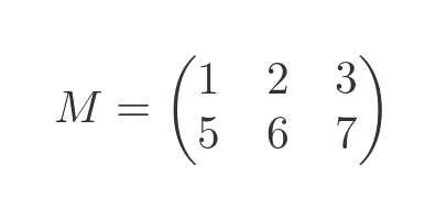
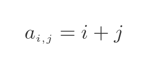
A matrix is a 2-dimensional array of numbers, for example:

This article gives a basic introduction to matrices, including their properties, some of the operations that can be carried out on matrices, some special types of matrices, and finally some examples of how matrices are used, particularly in mathematics and computer science.

Shape of a matrix

The most obvious property of a matrix is its shape. The shape of a matrix is defined by the number of rows and the number of columns. For example, the matrix above is a 2 by 3 matrix, because it has 2 rows and 3 columns.

The shape of a matrix is sometimes called its size. The two terms are interchangeable

Note that the row, column order used in matrices is different to the x, y order we often use in maths.

The individual elements are also numbered in row, column order, as shown here:

Element a(2, 0), for example, is the element in row 2, column 0.

Special matrix shapes

Some particular matrix shapes are very useful.

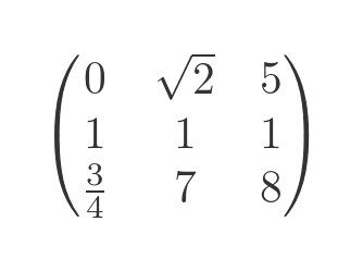
A square matrix has the same number of rows and columns. For example a 2 by 2 matrix, a 3 by 3 matrix, and so on. Here is an example 3 by 3 matrix:

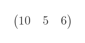
A row matrix is a matrix with only 1 row. This is useful because it can be used to represent a vector in matrix form:

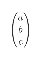
A column matrix is a matrix with only 1 column. It can also be used to represent a vector in matrix form:

If we multiply a vector (in matrix form) by a square matrix of equivalent size, it transforms the vector. This is very useful in many fields, including computer graphics. We can freely swap between row or column forms as required to allow the matrix multiplication, as described below.

Also, if we multiply a row and column matrix, we obtain the dot product of the two vectors.

It is possible to define a matrix that is infinite in one or both directions. For example, this matrix is based on the equation:

If we allow i and j to take every value from 0 and infinity, we create a matrix that has a countably infinite number of rows and columns:

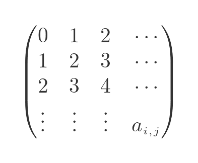
This matrix is well-defined, and we can perform certain operations on it. For example, we can add it to another infinite matrix, or we can multiply it by a scaler.

It is also possible to define a matrix that has zero rows or columns. To see how that makes sense, consider this 2 by 2 matrix:

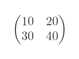
If we remove the leftmost column, we get a 2 by 1 matrix:

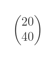
What if we remove the leftmost column again? Clearly, it is possible to do this, and logically this should give us a 2 by 0 matrix. Such a matrix has no elements, but it could still be said to have a shape.

What if we try to remove the leftmost column again? Well, obviously we can't because there is no leftmost column. We can't have a 2 by -1 matrix!

Why are zero-size matrices useful? A helpful analogy might be the idea of zero factorial. When we look at certain series, such as Maclaurin series, it is often useful to define the factorial of zero to be equal to 1. This is useful because we can define the terms in the series as an infinite sum, without having to make a special case for n = 0. Zero dimension matrices fulfil a similar role in matrix algebra.

Special matrix values

Certain square matrices have special properties. We will use 3 by 3 matrices for illustration.

A zero matrix (or null matrix) contains all zeros:

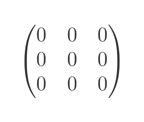
If we add a zero matrix to another matrix, the other matrix is unchanged. If we multiply any matrix by a zero matrix, the result is a zero matrix.

A unit matrix (or identity matrix) contains all zeros, except that the leading diagonal is all ones:

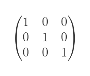
If we multiply any matrix by a unit matrix, the other matrix is unchanged.

A scalar matrix contains all zeros, except that the leading diagonal elements all have the same value S:

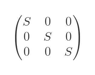
If we multiply any matrix by a scalar matrix, every element of the other matrix is multiplied by S.

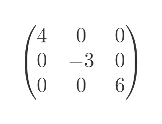
A diagonal matrix contains all zeros except that the elements of the leading diagonal can be any value:

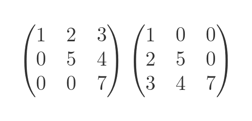
A symmetric matrix has elements that obey the equation:

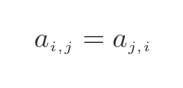
This means that the matrix is symmetrical about the leading diagonal:

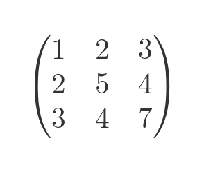
If we transpose a symmetric matrix, the result is identical to the original matrix.

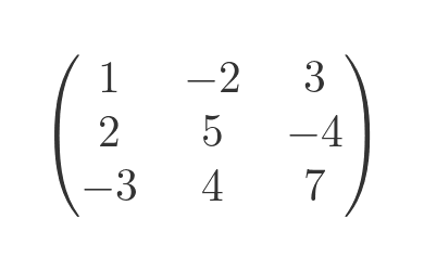
A skew-symmetric matrix has elements that obey the equation:

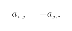
This means that a term on one side of the leading diagonal is the negative of its reflection over the diagonal line, like this:

A triangular matrix is where all elements on one side of the leading diagonal are zero. There are two types of triangular matrix:

• In an upper triangular matrix the values below the diagonal are zero. The values above the diagonal are not necessarily zero (although some or all of them might be). This is shown on the left below.
• In a lower triangular matrix the values above the diagonal are zero, and the values below the diagonal are not necessarily zero. This is shown on the right below.

Operations on matrices

We can carry out various operations on matrices such as addition (and subtraction), multiplication, transposition, finding the determinant, and inversion. We won't go into great detail about these operations, as this article is only an overview of matrices.

Matrix addition and subtraction

To add two matrices, they must both be the same shape. The resulting matrix is obtained by adding the matrices, term by term. For example:

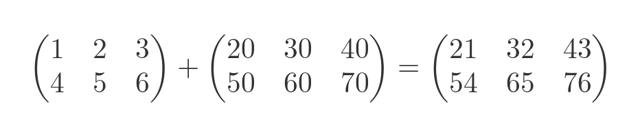
For instance, looking at the term (0, 0) in each matrix, this term is 1 in the first matrix, 20 in the second matrix, and 21 in the result matrix. Matrix subtraction works in the same way, but of course, we subtract the terms of the second matrix from the terms of the first matrix.

Matrix scalar multiplication and division

There are two ways to multiply matrices. We can multiply a matrix by a scalar, or we can multiply 2 matrices together.

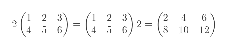
Multiplying a matrix by a scalar simply involves multiplying each term in the matrix by that scalar. This operation is commutative, that is M times a equals a times M:

It is also possible to divide a matrix by a scalar, by dividing each term in the matrix. It isn't possible to divide a scalar by a matrix, although it is possible to multiply a scalar by the inverse of a matrix (see below).

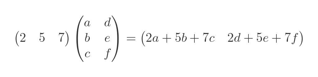
Multiplying two matrices

We can multiply 2 matrices, but the process is slightly more complex than scalar multiplication. We will start with a simple case:

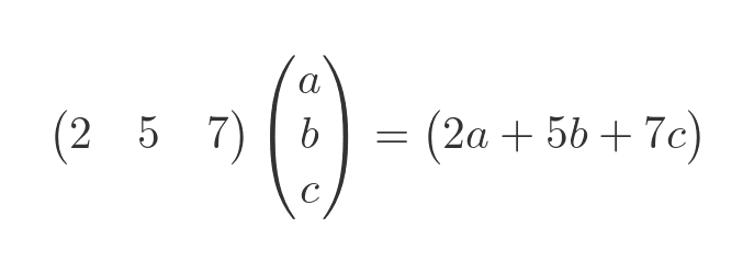
We take each element in the row of the first matrix and multiply it by the equivalent element in the column of the second matrix. The result is a linear equation, where the coefficients are specified by the first matrix and the values are specified by the second matrix. The result is created as a 1 by 1 matrix. If the second matrix contained numbers, rather than x, y and z, the result matrix would contain the numerical result of the linear equation.

To multiply 2 matrices, the number of columns of the first matrix must be equal to the number of rows of the second matrix.

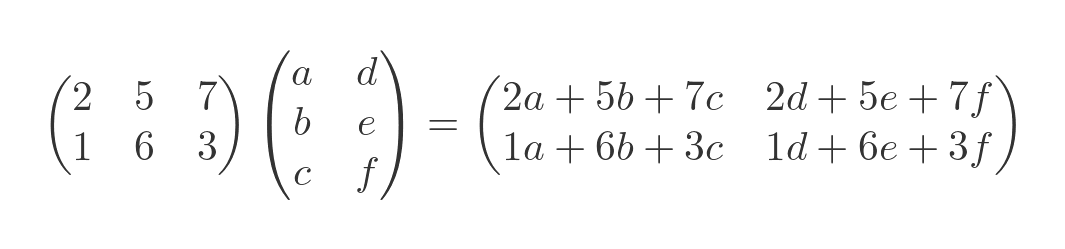
Here is what happens if we add an extra column to the second matrix:

This time, we perform a row-by-column multiplication between the first matrix and the first column of the second matrix. This becomes the first element of the result. We also perform a row-by-column multiplication between the first matrix and the second column of the second matrix. This becomes the second element of the result.

In effect, matrix multiplication is calculating the linear equation twice, with 2 different sets of values.

We can also add an extra row to the first matrix, which represents a second linear equation. This time the result is a 2 by 2 matrix that shows the result of applying each linear equation to each set of values:

Transposing matrices

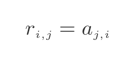
To transpose a matrix, we swap the row and column indices of each element:

This, effectively, reflects the matrix over its leading diagonal. The transposed matrix also swaps width and height compared to the original matrix, which means it has a different shape (unless the matrix is square):

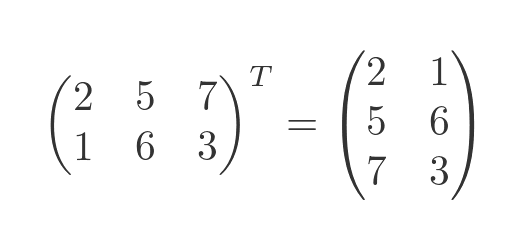
A superscript T is often used to indicate transposition, as shown in the formula.

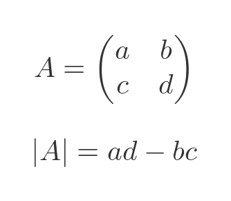
Determinant of a matrix

The determinant of a matrix is a single scalar value that is calculated from all the elements of the matrix. It only exists for square matrices. The determinant is used in calculating the inverse of a matrix and is also useful when solving simultaneous equations using matrices. If a matrix is used to specify a geometric transformation, the determinant relates to the scale factor of the transformation.

The determinant can be thought of as the "magnitude" of the matrix. The determinant of a matrix A is written as:

For a 2 by 2 matrix, the value is calculated like this:

The formula for the determinant of 3 by 3 or larger matrices follows a recursive pattern. We won't cover it here.

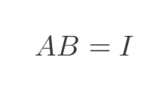
Inverse of a matrix

A matrix is invertible if it is a square matrix, and if its determinant is not zero.

If matrix A is invertible, its inverse is the matrix B such that:

The inverse of A can be written as:

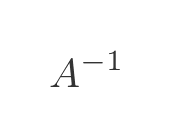
The inverse of a matrix is very useful. For example, if A represents a geometric transform, then the inverse of A will undo that transform.

Applications of matrices

Matrices are useful for solving systems of linear equations, and for representing transformations between vector spaces.

Complex numbers can be represented in an alternative form, as 2 by 2 matrices. This is useful when considering quaternions and other extensions of complex numbers.

They are useful for modelling data. For example, a matrix can be used to model temperature, fluid flow, etc. at different points in a system. Computations can then be applied to the data using matrix algebra. Modelling has uses in many branches of physics and engineering, and other areas such as economics.

In computer science, matrices are used extensively in computer graphics. They are used for 2D graphics (for example word processing and drawing software) and 3D graphics (for example, computer games). We use adjacency matrices to model graphs in computer science. Matrices are also used in colour management, for example in the print industry to ensure that the colours the designer sees on their computer screen will match the colours of the final printed product.

Other types of matrices

We have only discussed 2-dimensional matrices here. Matrices can also exist in 3 or more dimensions.

All the matrices above have real number elements. It is also possible for a matrix to contain complex numbers.

Extending this further, we can also have a matrix of vectors - for example, we might use a 3D matrix to model the atmosphere, where each element is a vector representing the wind strength and direction.

It is also possible to have a matrix of matrices, where each element of the main matrix is also a matrix.

See also

• Determinants
• Matrix inverse
• 2D transformation matrices
• Solving simultaneous equations with matrices
• Introduction to eigenvectors