Calculating a Maclaurin series

A Maclaurin series allows us to calculate the approximate value of a function f(x) as a polynomial:

The values a₀, a₁, a₂ ... can be calculated in terms of the derivatives of the function at x = 0:

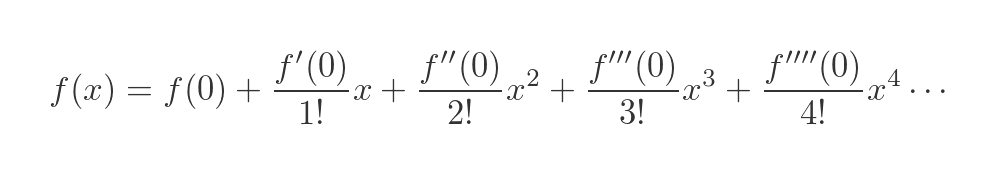
In this formula:

• f(0) is the value of the function for x = 0.
• f'(0) is the value of the first derivative function for x = 0.
• f''(0) is the value of the second derivative function for x = 0.
• f'''(0) is the value of the third derivative function for x = 0.
• And so on.

The method can be applied to many common functions, for example the exponential function e^x, the natural logarithm ln(x), sine and cosine functions, hyperbolic sine and cosine functions, and many others.

The result is often a polynomial with an infinite number of terms. In many common cases, the terms get smaller very quickly for higher powers of x, so it is possible to calculate a value to any required accuracy by calculating the values of a sufficient number of terms.

The Maclaurin series approximates the value of the function at x = 0. It also works well for values of x that are close to zero. For values of x that are far away from zero, it is generally necessary to calculate more terms to obtain the required accuracy.

A Taylor series, which is a generalisation of the Maclaurin series, can be used to calculate accurate values of f(x) when x has a value other than zero. That will be covered in a later article.

How the Maclaurin series works

We are trying to express some function f(x) as a polynomial of the form given above. We aim to make this approximation as accurate as possible for values of x that are close to 0.

We will start by assuming that it is possible to find such a series.

We can then apply a process to find the values of a₀, a₁ etc.

Finally, we can verify that the method works for a particular f(x) by creating a graph of the polynomial, and comparing it to a graph of tf(x).

Step 1 - finding the value of a₀

Given the approximation we defined above:

We can determine the value of a₀ quite easily. If we set x to zero, all the terms in x go to zero, so we are left with:

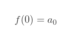
So the value of a₀ is simply f(0).

Step 2: finding the value of a₁

Looking again at the original formula:

How can we find the value of a₁? We can do this by differentiating each side. Since f(x) and the infinite polynomial are supposed to be the same function, it follows that the first derivatives should also be equal.

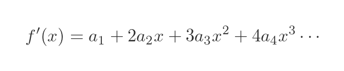
We have just used the power rule to differentiate the RHS of the equation:

• The derivative of a₀ is zero, so the term in a₀ disappears.
• The derivative of a₁x is a₁.
• The derivative of a₂x² is 2 a₂x.
• The derivative of a₃x³ is 3 a₃x².
• And so on.

As before, we set x to zero. all the terms in x go to zero, so we are left with:

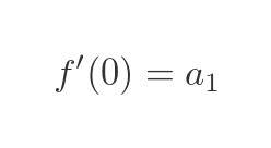
This tells us the a₁ is equal to the first derivative of f(x) for x = 0.

Step 3 - finding the value of a₂

Here is the previous formula, where we differentiated each side:

Now we would like to find the value of a₂? We could try differentiating each side again since it worked quite well last time. The same logic applies - since f(x) and the infinite polynomial are the same function, it follows that the second derivative should also be equal.

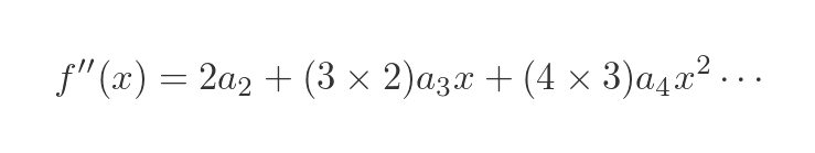
We use the power rule to differentiate the RHS of the equation, but this time we need to take into account the factors from the previous time:

• The derivative of a₁ is zero, so the term in a₁ disappears.
• The derivative of 2 a₂x is 2 a₂.
• The derivative of 3 a₃x² is (2 × 3) a₃x.
• And so on.

Now we can set x to zero again, and once again all the terms in x will be zero, so we have:

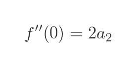
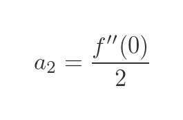
Which gives us this value for a₂:

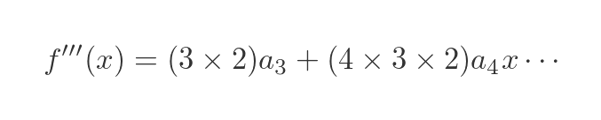
Step 4 - finding the value of a₃

To find the value of a₃ we just need to repeat the previous procedure.

Taking the previous equation:

Differentiating once more gives:

When x = 0 we have

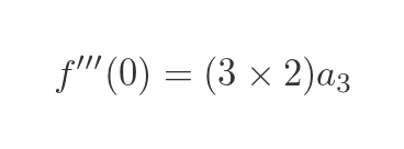
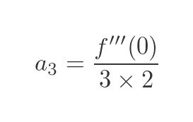
Which gives us this value for a₃:

General formula for a Maclaurin series

There is a pattern here that we can use to extend the series to any number of terms. The nth term is equal to the nth derivative of f(x) divided by a factor. We need to know how to calculate the factor.

a₃ has a divisor of 6 because we differentiated the term 3 times, first as a cube (giving a factor of 3), then as a square (giving an extra factor of 2), then as a term in x (giving an extra factor of 1, which has no effect).

The divisor is therefore (3 × 2 × 1), which is 3 factorial.

For a₄, there is an extra step of differentiating the power of 4, which gives an extra factor of 4. So the divisor for a₄ is 4 factorial. For a₅ the divisor is 5 factorial, and so on. So we can write the general series as:

This can be written as a sum, using sigma notation:

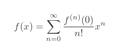
There are a couple of things to note about this equation:

• f⁽ⁿ⁾ means the nth derivative.
• f⁽⁰⁾ therefore means the zeroeth derivative, which is simply the function itself, f.
• 0 factorial is defined to have a value of 1.

See also

• Maclaurin series of the exponential function
• Maclaurin series of the sine function
• Pi isn't about circles