Introduction to eigenvectors

The product of a square matrix A and a column vector v is a new column vector. The new vector will normally have a different direction from the original, with the matrix representing a linear transformation. However, certain vectors will keep their original direction. We say that such a vector is an eigenvector of the matrix A.

In this article, we will look at eigenvectors, eigenvalues, and the characteristic equation of a matrix. We will also see how to calculate the eigenvectors and values of 2- and 3-dimensional square matrices.

2D example

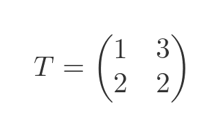
Consider this matrix, T:

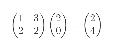
If we multiply this matrix by the vector (2, 0) we get a new vector (2, 4):

This is illustrated below. The left-hand plot shows the original vector (2, 0) in cyan. It shows several other vectors in different colours. The right-hand graph shows the same set of vectors transformed by the matrix T above:

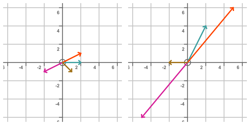
Generally, each transformed vector on the right has a different size and direction compared to its untransformed counterpart on the left.

There are two special vectors that do not change direction when transformed by T. Those vectors are (1, 1) and (-3, 2):

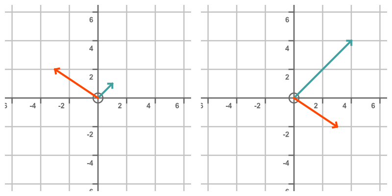
These vectors are called the eigenvectors of T. The cyan vector (1, 1) is transformed into the vector (4, 4). The transformed vector points in the same direction as the original, but it is 4 times longer. We say that the vector (1, 1) is an eigenvector of T with an eigenvalue of 4.

The orange vector (-3, 2) is transformed into the vector (3, -2). It appears to be pointing in the exact opposite direction to the original, but one way to describe that is to say that it has the same direction but with a negative length. Vector (3, -2) is equal to (-3, 2) multiplied by -1, so we say this vector is an eigenvector of T with an eigenvalue of -1.

Eigenvector definition

We can define an eigenvector using this equation:

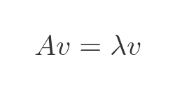
Here A is a square matrix of order n (the above example was a square matrix of order 2), v is a vector also of order n, and λ is a scalar constant value.

We say that v is an eigenvector of A and λ is an eigenvalue of A corresponding to eigenvector v.

Usually, the number of eigenvalues will be equal to the order of the matrix (so in the previous example, there were two eigenvalues because it was a two-by-two matrix). Each eigenvalue will be associated with an eigenvector, but bear in mind that if v is an eigenvector then any scaler multiple of v will also be an eigenvector. It is only the direction of the vector that matters.

Also, there are sometimes degenerate cases. For example, a two-by-two matrix might only have one eigenvalue that corresponds to two different eigenvectors that are not collinear.

The characteristic equation

If we take the previous equation for the eigenvector, we can use it to find the eigenvalues. Here is the equation from earlier:

We will make use of the identity matrix. This is a square matrix where every element of the leading diagonal is 1, and all the other elements are 0. If we multiply any vector v by an identity matrix of the same order, it leaves the vector unchanged:

So we can replace v on the RHS of the original equation with Ix and the equation will still be valid:

We can rearrange this by moving both terms to the RHS and taking out a common factor of v. Note that, in the equation below, 0 represents a zero vector rather than the scalar value 0. For example, it would be (0, 0) if v has order 2:

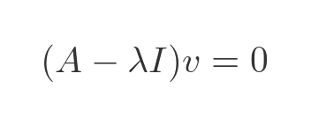
This says that the matrix (A - λI) always takes v to 0, which implies that the determinant must be 0. So:

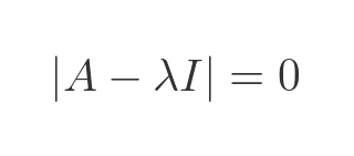
This is called the characteristic equation of A. We won't prove it here, but the solutions to this equation give the eigenvalues of A, and from the eigenvalues we can find the eigenvectors.

Finding the eigenvalues of a two by two matrix

Let's use this to find the eigenvectors of our previous example matrix:

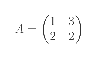
Here is the characteristic equation using this matrix and the identity matrix of order 2:

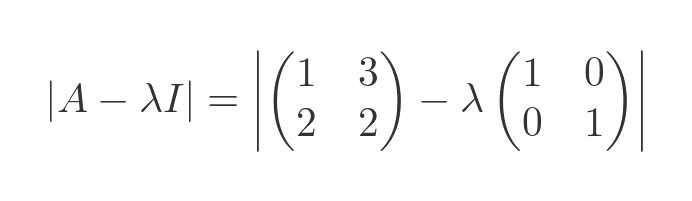
We multiply the identity matrix by λ:

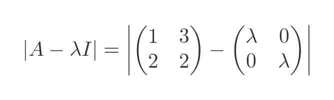
And subtract the two matrices:

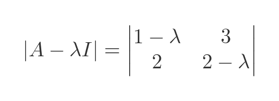
Here is the equation for the determinant of a two by two matrix:

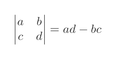
Applying this to our matrix gives:

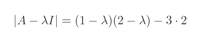
We will skip the simplification steps, but we end up with:

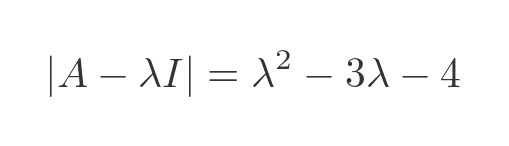
This is a quadratic equation. We can use the quadratic equation to find the following two solutions:

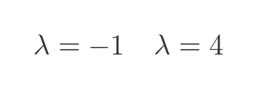
These are our eigenvalues.

Finding the eigenvectors from the eigenvalues

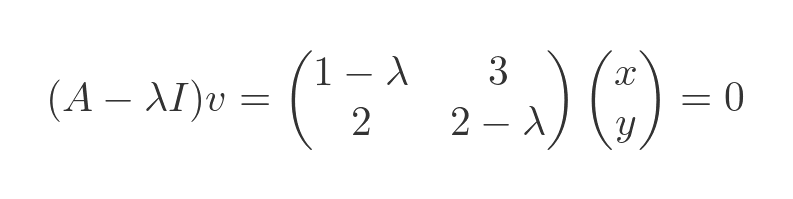
To find the eigenvectors, we return to the earlier equation:

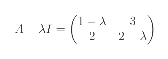
We previously found an expression for A - λI:

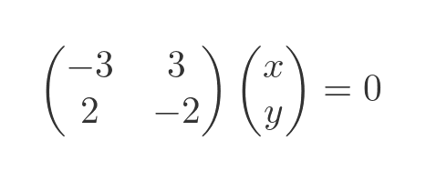
Substituting this into the previous equations, and representing v as a column vector (x, y), gives:

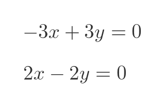
We already know that the two eigenvalues are -1 and 4. If we substitute -1 for λ we get:

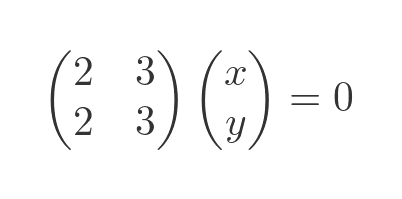
Multiplying out the matrix gives two simultaneous equations:

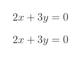
Now these two equations are collinear (in fact, they are identical), so they do not have a unique solution. They are solved by any v that satisfies the relationship:

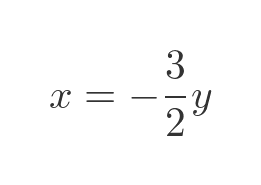
This is the equation of a straight line, passing through the origin, with a slope of -2/3. Our eigenvector is any vector on that line.

Right at the start, we demonstrated graphically that the vector (-3, 2) was an eigenvector, and this equation validates that. But we also saw that any vector with the same slope is also an eigenvector. So for example, (-6, 4) is an eigenvector (and it also satisfies the same relationship). There are infinitely many vectors with different lengths but the same slope. We could choose any vector, but it is common to choose the smallest vector that has integer components (if that vector exists).

We can do the same with λ equals 4:

This gives the following two simultaneous equations:

These are solved by any pair of values that satisfy:

This again is a straight line, passing through the origin, with a slope of 1. So (1, 1) is an eigenvector, so is (2, 2) etc.

Solving a three-by-three matrix

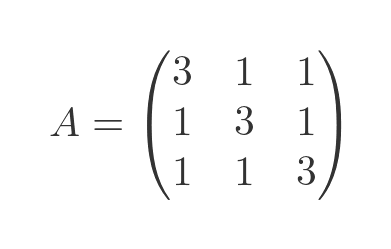
Now let's try a three-by-three matrix. The steps can be quite lengthy, so we will skip the detailed arithmetic in some places. We will use this matrix:

The determinant of the characteristic equation is:

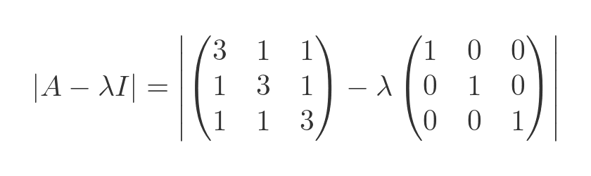
Adding the two matrices yields:

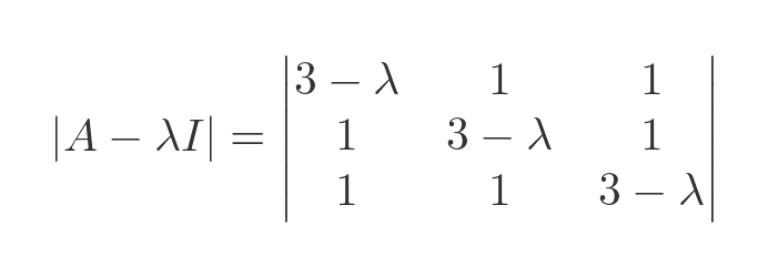
We will use the standard equation for a three-by-three determinant:

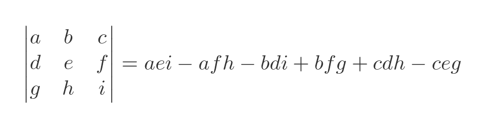
Substituting the values from the matrix, after some tedious gathering of terms, gives us:

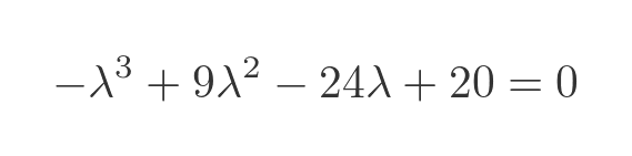
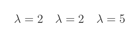
This has three solutions (that can be verified by substituting λ in the equation above), but two of the solutions are equal to 2:

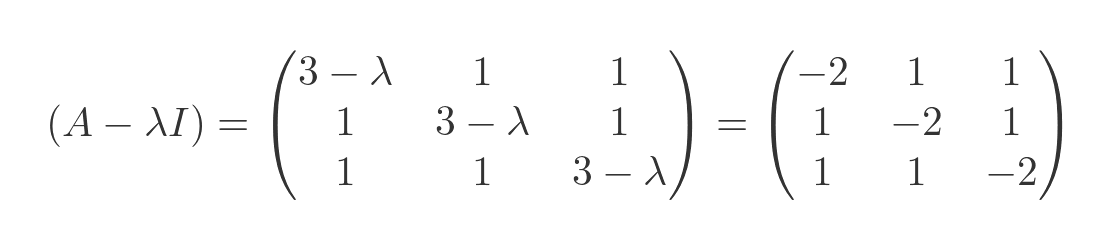
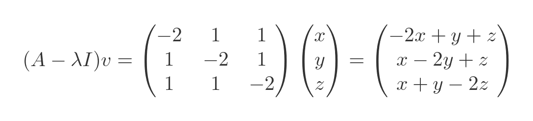
Next, we will find the eigenvectors. As before, we substitute the known λ values into the matrix, multiply by v and solve for zero. We will start with λ equal to 5. This gives the following matrix:

Multiplying this by a 3-vector (x, y, z) gives:

This is equal to zero when:

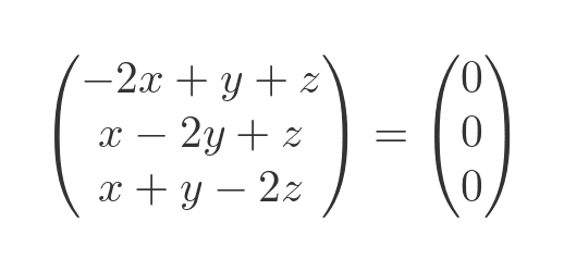
This gives us a set of simultaneous equations:

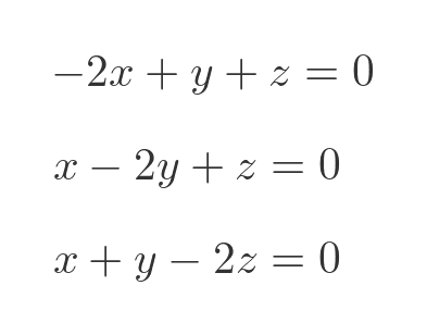
Subtracting the second equation from the first gives:

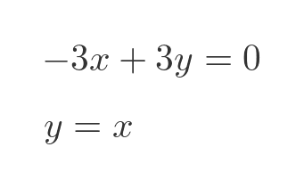
Subtracting the third equation from the first gives:

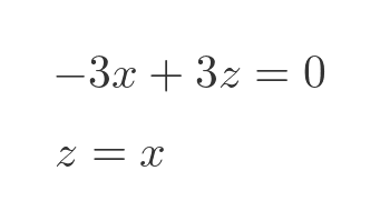
For any given x we can find a value for y and z, so these linear equations specify a straight line. The eigenvector is any vector collinear with this line. If we arbitrarily pick 1 for x, then y and z are also 1, so the eigenvector associated with eigenvalue 5 is (1, 1, 1).

Now let's try again with the other λ value, 2:

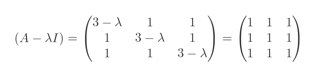
Multiplying by v:

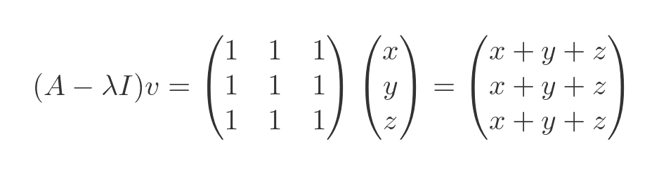
This, again, is equal to zero when:

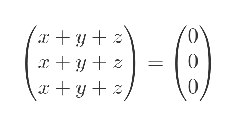
All the lines of the matrix are identical, so rather than a set of simultaneous equations, we get the same equation repeated three times:

We can solve for z:

You might recognise this as the equation of a plane. We won't prove it here, but the reason we get a plane in this case is that the λ value of 2 appears twice as an eigenvalue.

To fully specify a plane, we need to know two vectors on the plane. When we had a line, we knew the direction of the vector but we had the freedom to choose its length. But in a plane, we get to choose the direction and the length of our two vectors (both vectors must be on the plane, and they can't be parallel to each other).

Let's arbitrarily select x as 1 and y as 0. According to the formula, this makes z equal to 1. So one of the eigenvectors is (1, 0, -1).

For the second vector, it would be nice if it were orthogonal to the first vector. One way to do this is to keep x as 1 and choose y as -1. This gives z a value of (1, -1, 0).

We could have set y equal to 1 instead, but then z would have been -2, which is fine but not quite as nice. In fact, we could have used any linear combination of the two vectors (1, 0, -1) and (1, -1, 0), they all exist on the same plane.

See also

• What is a matrix?
• Determinants
• Matrix inverse
• 2D transformation matrices
• Combining and inverting transform matrices
• Solving simultaneous equations with matrices