Solving simultaneous equations with matrices

A system of simultaneous equations is a set of two or more equations that share the same variables. We solve the equations by finding a common set of values of the variables which solve all the equations at the same time.

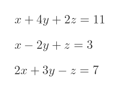
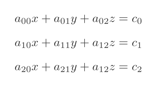
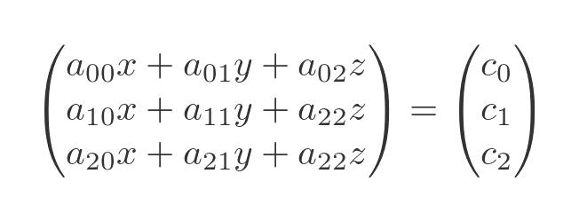
In this article we will only consider linear simultaneous equations, that is a system where each of the equations is a combination of the variables multiplied by constant coefficients. For example, here is a system of linear equations of three variables:

There are various ways to solve simultaneous equations, but in this article, we will see how to use matrices to find a solution. Unlike the ad hoc methods we normally apply to solve simultaneous equations of two or three variables, the matrix method is easy to implement in code, so we can use computers to solve very large systems of equations.

Example - 2 variables

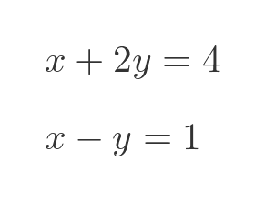
Here is a simple set of two simultaneous equations:

One way to solve these equations is to eliminate one of the variables. We can do this, for example, by subtracting the second equation from the first:

We subtracted the left-hand sides and the right-hand sides. Since the LHS equals the RHS for both original equations, it follows that the LHS and RHS of the difference equation will be equal to each other. Simplifying the equation above gives:

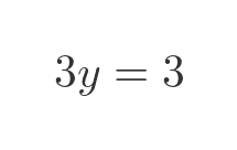
This tells us that y is 1, We can substitute this value of y into the first original equation:

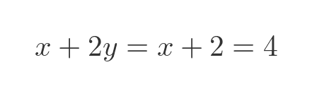
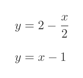
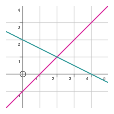
This tells us that x is 2, so we have solved the equations. An alternative way is to graph the two equations. We can rewrite the two equations to give y as a function if x:

Plotting these two functions shows that they meet where x is 2 and y is 1, which is the same solution as before:

Solving the problem with matrices

The solution above works well when we have two equations involving two variables. It also is possible to solve systems of three equations with three variables using the same technique. But if we need to solve systems of four, five, six or more variables it is a laborious process. We need to inspect the equations and make a decision on what steps to take based on the values of the coefficients.

What we really need is a mechanical process that we can hand over to a computer to solve. Matrices provide that. If we express the coefficients of a simultaneous equation in matrix form, we can solve the equations using basic matrix operations. This process can be automated quite easily using existing matrix manipulation software. We will go through the process here without proof, but we will go on to prove it later.

One thing to bear in mind is that the number of calculations increases as the factorial of the number of equations. Factorials get very big, very quickly. An ordinary office computer might solve a system of ten equations quite quickly, but a system of twenty equations would take almost a million million times as long (literally), which at the time of writing would take a long time on even the fastest supercomputer. A system of thirty equations would be completely impossible using this method. There are alternative methods for solving large systems, but we won't cover them here.

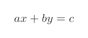
We need to write our two equations in a standard form:

Here are the two equations from earlier in this form:

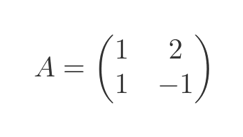
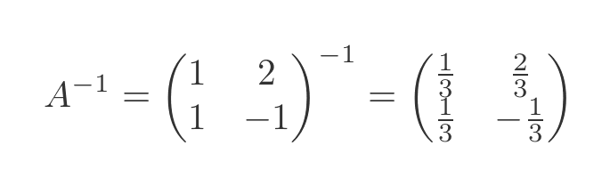
We then need to form two matrices. The first, A, contains the factors of x and y for each equation:

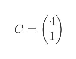
The first matrix, C, contains RHS for each equation:

Now we need to find the matrix inverse. This is a standard calculation as described in the linked article. The result in this case is:

We can find the solution by multiplying the inverse of A by C:

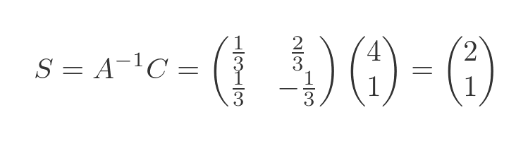
The resulting matrix, (2, 1), indicates that the solution has an x value of 2 and a y value of 1, exactly as we discovered earlier. The matrix method, however, doesn't require us to inspect coefficients. It is an automatic process.

Systems of 3 equations

Let's solve the 3 variable system we saw at the start of the article:

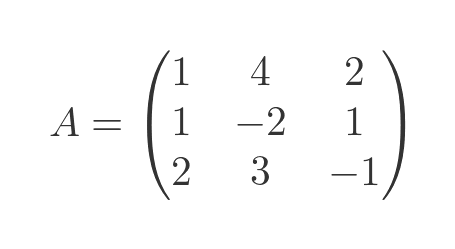
We can express the coefficients of these equations as a matrix A, just like the previous example:

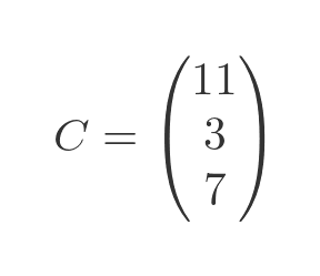
We can also examine the RHS as a column matrix C:

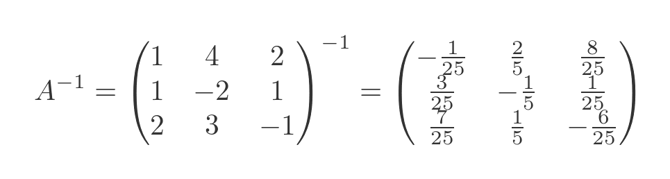
We need to find the inverse of matrix A. This can be done with any matrix calculator program (several are available online):

The solution, again, is found by multiplying the inverse of A with C:

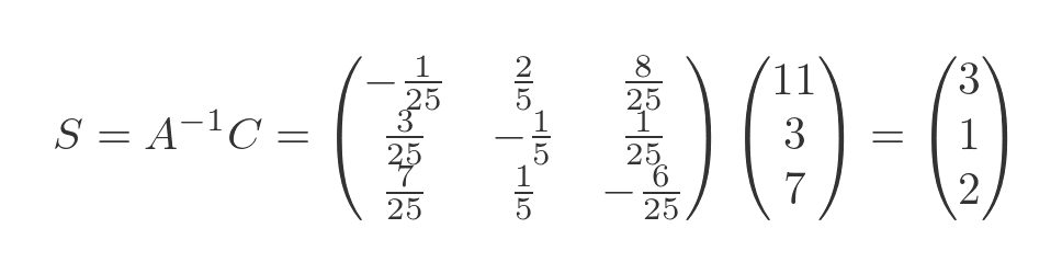
So the solution has x, y, and z values of 3, 1, and 2. We can verify these by plugging them back into the original equations:

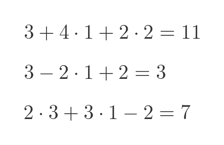
Both sides of each equation agree.

Proof

We will prove this for the case of a general set of three equations:

We will represent these equations using three matrices:

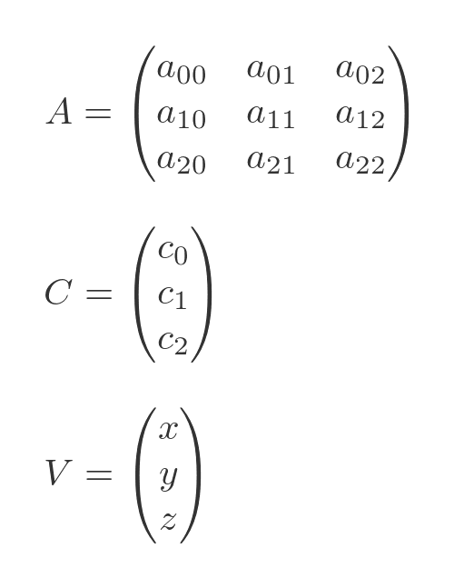
A holds the coefficients on the LHS, C holds the constants on the RHS, and V represents the variables x, y,and z.

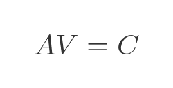
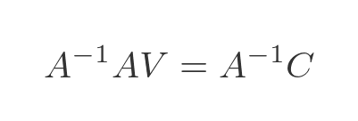
We will start by proving that, based on the original three equations, the following is true:

Substituting the matrix values gives:

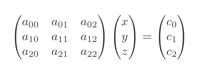
Multiplying out A and V gives:

The matrices are equal if and only if each of their corresponding terms are equal. Looking at the matrices, each element in AV is equal to the LHS of one of the original equations, and each element in C is equal to the corresponding element in C. Therefore:

This is the first step in our proof.

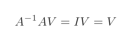
If we now multiply both sides with the inverse of A we get:

We know that the inverse of A multiplied by A gives the unit matrix. And we know that the unit matrix multiplied by any matrix V is equal to V. So we have:

Substituting this proves that:

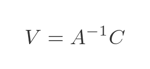
So if we multiply the inverse of A by C we get a column vector with values that correspond to the x, y, and z values that solve the equation. This proves what we previously demonstrated, giving us a method to solve simultaneous equations.

This proof can easily be adapted to any number of variables.

Equations with no solution

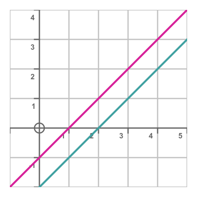
Sometimes a set of simultaneous equations has no solution. We will illustrate this with the two-variable case. Consider these equations:

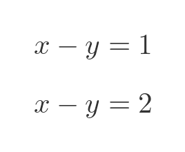
If we plot a graph of these two functions, we can see that the two lines are parallel. They don't intersect. There is no solution because there is no value of x and y that satisfies both equations:

Here is a slightly different case:

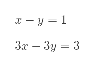
If we plot these two graphs, we see that they are both the same line:

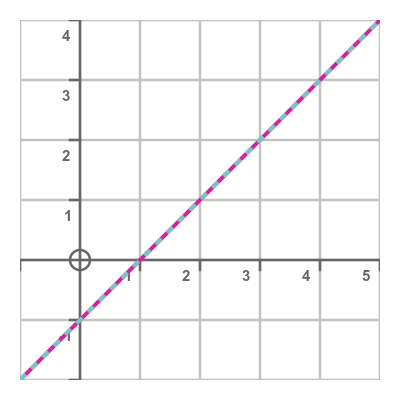
This is because both equations are one and the same. All the terms in the second equation are multiplied by 3, but the equation still describes the same line. This means that there is no unique solution to the equations. Every value of x is a solution, because for a given value of x, both equations will yield the same y value.

Both situations arise when the matrix isn't invertible. This occurs when the determinant of the matrix is zero. If the determinant is zero, then the simultaneous equations have no unique solution. They either have no solution at all, or they have an infinite number of solutions.

In the case of three variables, each equation defines a plane in 3D space. If those three planes intersect at one point, that point will be the solution of the equations.

In some cases, all three planes might be parallel to some particular line in space. In that case, each pair of planes will intersect, but there will be no point where all three intersect, so there will be no solution.

In other cases, all three planes might meet along a particular line in space. In that case, there will be infinitely many solutions, but no unique solution.

Similar situations are possible for higher-order systems of simultaneous equations. In every case, a determinant of zero indicates that there is no unique solution.

See also

• What is a matrix?
• Determinants
• Matrix inverse
• 2D transformation matrices
• Introduction to eigenvectors