Adjacency matrices

A graph is often represented by a graph diagram like the one on the left, below:

The same graph can be represented as an adjacency matrix like the one on the right. This matrix contains all the same information as the graph diagram but in a different form.

The graph diagram is usually easier to visualise, but the matrix form is useful because it can be analysed and manipulated mathematically. Since a matrix is simply a table of numbers, it can also be processed by a computer program.

In this article, we will look at adjacency matrices in detail, for different types of graphs. For more information on the different types, see the main graphs article.

Simple graph

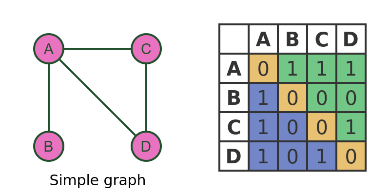
The graph above is a simple graph showing 4 vertices, with simple edges between the vertices. The matrix contains a 1 to indicate that two vertices are connected and a 0 to indicate that they are not connected.

For example, row A column B is set to 1 because there is an edge between vertices A and B. But row B column D is set to 0 because there isn't an edge between vertices B and D.

For brevity, we will write row A column B of the matrix as M[A, B].

It is interesting to note that all elements on the leading diagonal (shaded yellow) are zero because no vertex is connected to itself. For example M[A, A] is set to 0 because A is not connected to itself.

Notice also that the matrix is symmetrical about the leading diagonal, i.e. the area shaded in blue is a reflection of the area shaded in green. This is because, in a simple graph, every edge works in both directions. For example, if A is connected to B, this means that B is connected to A (by the same edge).

Simple graph with loop

This graph is identical to the previous one, except that it has a loop on vertex C (i.e. C is connected to itself):

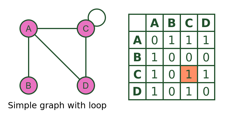
The only difference is that M[C, C] is now set to 1 to represent the loop.

Directed graph

This diagram represents a directed graph. In a directed graph, each edge is one-directional, for example there is an edge from W to X but no edge from X to W:

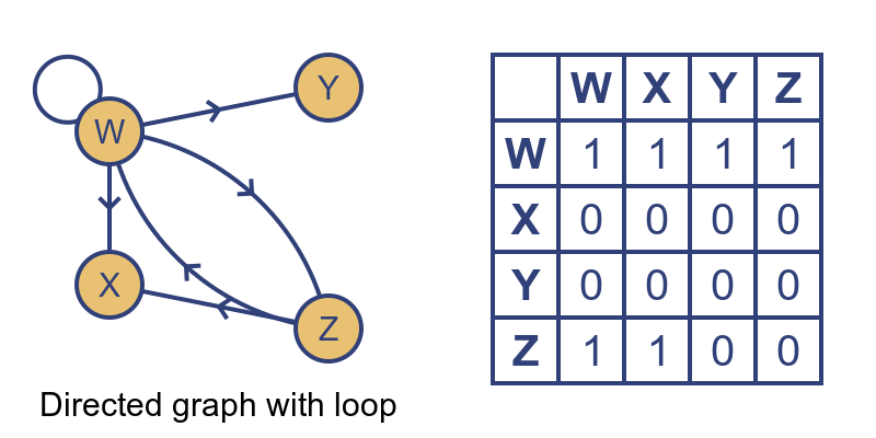
A directed graph, is not necessarily symmetrical about the leading diagonal, because an edge in one direction doesn't necessarily imply an edge in the opposite direction.

Where the connection is bidirectional, it is indicated by two edges, one in each direction (for example the edge between W and Z is bidirectional). In that case, there is a 1 in both positions in the matrix (M[W, X], and M[X, W]).

We have also shown a loop - vertex W is connected to itself. This is indicated by a 1 in M[W, W]. Even in a directed matrix, a loop has no direction. The loop connects W to W, so it doesn't have a direction.

Multigraph

A multigraph allows for more than one edge between two vertices. It can be directed or undirected, but in this example, we will only look at the undirected case:

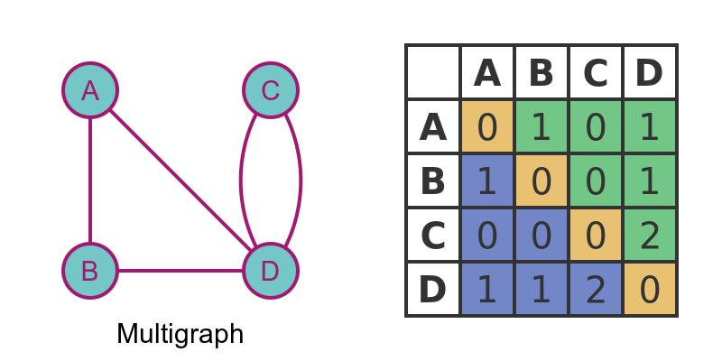
In this case, there are 2 edges between C and D. The adjacency matrix is slightly different to the simple graph because the entry shows the number of edges. So M[C, D] and M[D, C] are both equal to 2.

If two vertices have no edge between them, the value is 0 (similar to a simple graph). For example M[A, C] is zero because A and C are not connected.

This matrix is symmetric because it represents an undirected graph. If it was a directed graph, the matrix could be asymmetric.

The leading diagonal is all zeroes unless the graph has loops. This again is similar to a simple graph.

Weighted graph

In a weighted graph, each edge has a value associated with it, called a weight. Weighted graphs can also be directed or undirected, but again we will only look at the undirected case:

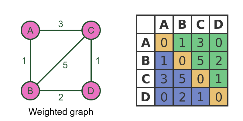
The adjacency matrix contains the weight of the edge, for example, M[A, C] and M[C, A] are both 3, because the edge between A and C has a weight of 3.

We need to use a special value to indicate the case where there is no edge. In this case, we are using the value 0 to indicate no edge, on the assumption that if there is an edge its weight it cannot be 0. For example, if the graph represents a road network and the weights indicate distances, it is reasonable to say that no road can have a length 0, so we can use 0 to indicate that no road exists at all.

In some systems it might be valid to have an edge with a weight of 0. In that case, it would be necessary to choose some other value to represent no edge (for example -1 if negative weights are not valid).

Weighted multigraphs cannot be easily represented as adjacency matrices because a pair of vertices can have multiple values.

Vertex properties

We can use the adjacency matrix to deduce various properties of a vertex. The section below applies to simple graphs. The techniques can be adapted for directed, weighted or multi-graphs, but we will not cover that here. We will use this simple graph:

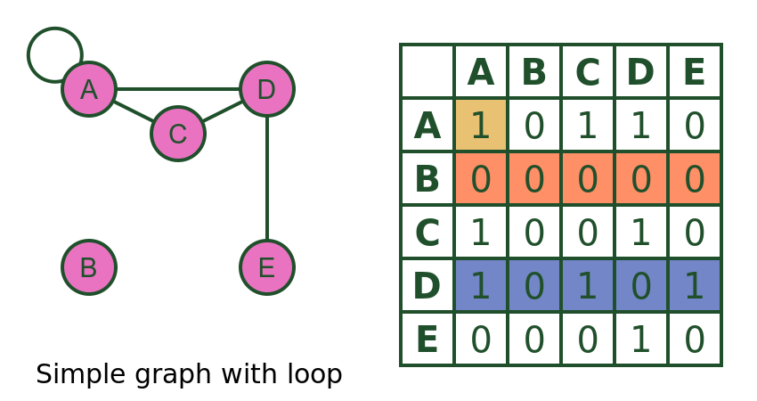
As we have noted before, the leading diagonal indicates whether the graph has loops. in this case M[A, A] is non-zero, so vertex A has a loop.

We can also easily check the degree of a vertex (the number of edges that connect to it). We can do this simply by adding up the number of ones in the row for that vertex (we could use the column instead, as the matrix is symmetric).

For example, vertex D has a degree of 3, because there are 3 ones in row D (marked in blue).

Vertex B has degree 0, because there are no ones in row B (marked in orange). This means that vertex B is disconnected. Looking at the graph diagram confirms this.

Vertex A is a special case because it has a loop. A loop counts as 2 connections because it joins the vertex twice. When we add up the number of ones in a row, we need to add 2 if the leading diagonal element is set. In this case A has order 4.

Graph properties

We can use the adjacency matrix to determine the properties of the graph as a whole. Again we will only consider simple graphs here, but the techniques can be adapted for other types.

A complete graph is a graph where every vertex is connected to every other vertex:

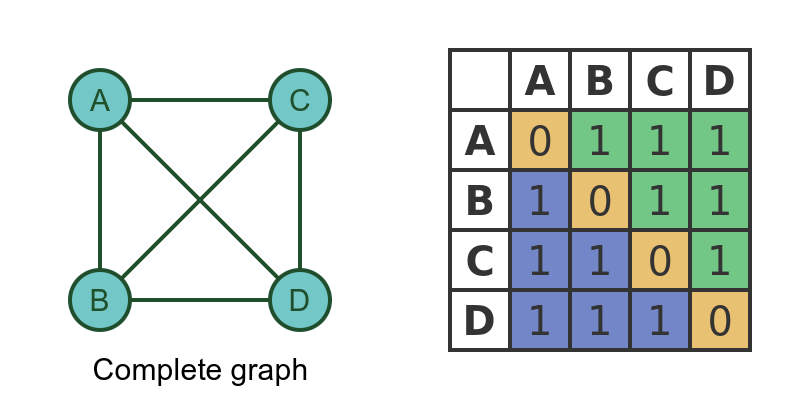
For a complete graph, every element of the matrix must be non-zero, except for the leading diagonal. This then means that there is an edge between every pair of vertices.

It is possible to use the adjacency matrix to determine other properties of a matrix, for example, if it is a tree, connected, bipartite etc. These properties are determined by simple algorithms that can be executed on the matrix. They will be covered in a separate article.

Computations on adjacency matrices

Finally, below are a couple interesting matrix calculations can be carried out on adjacency matrices. We will look at these in more detail in a future article.

Isomorphic graphs and permutation matrices

Two graphs G and H are said to be isomorphic if they are equivalent graphs that differ only because the vertices are named differently, and/or they are laid out differently:

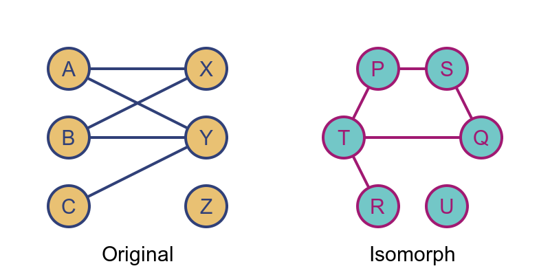
If we look at the adjacency matrices of two isomorphic graphs, they are identical except that the rows and columns might be in a different order between the two.

A permutation matrix is a special matrix that has the effect of reordering the rows and columns. For any 2 isomorphic graphs, the 2 matrices can be made identical by applying a suitable permutation matrix to one of the graphs.

Powers of the adjacency matrix

The adjacency matrix of a simple graph can be interpreted as follows: M[i, j] is 1 if there is a path between vertex i and vertex j.

The square of the adjacency matrix (i.e. the matrix multiplied by itself) has another interesting property. M²[i, j] is equal to the number of possible walks between vertex i and vertex j that have a length of exactly 2.

The cube of the adjacency matrix follows a similar pattern. M³[i, j] is equal to the number of possible walks between vertex i and vertex j that have a length of exactly 3. And so on.

Notice that this applies to walks, not paths. A walk is a route between 2 vertices that is allowed to visit the same vertex twice. So, for example, if there is an edge between vertices A and B, there will be a walk of length 1 from A to B. But there will also be a walk of length 3 which goes from A to B, then back to A, then back to B.

See also

• Graphs
• The seven bridges of Königsberg
• Dijkstra's algorithm
• Travelling salesman problem