Square root of 2 by 2 matrix using Cayley–Hamilton theorem

The square of a matrix R is just R multiplied by R. We can define the square root of a matrix as the inverse function, like this:

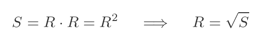
That is, if S is the square of R, then R is the square root of S. And just like regular square roots, a matrix can have more than one square root.

One important thing to notice is that R and S must both be square matrices, with the same shape. R must be square because only a square matrix can be multiplied by itself. And a square matrix multiplied by itself creates a matrix of the same order, so S must be square and of the same shape as R.

There are various ways to find the square root of a matrix, but for the case of a 2 by 2 matrix, there is actually a fairly simple formula we can use. We will introduce that formula here and then derive it.

Formula for the square root of a 2 by 2 matrix

The square root R of a 2 by 2 matrix S can be written as:

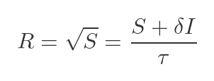
Where:

And:

In these formulas, |S| is the determinant of S, Tr(s) is the trace of S, and I is the unit matrix (see the next section for a recap of what these terms mean).

Notice that both terms are square roots, and the positive and negative values each give a valid solution. This means that a 2 by 2 matrix might have up to 4 square roots. However, sometimes multiple roots might have the same values, leading to fewer than 4 distinct roots.

Some useful values

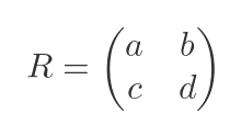
We will start by calculating some values that will be useful in deriving the formula. First, let's name the elements of the 2 by 2 matrix R:

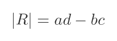
The determinant of a matrix is a single number that is calculated from the elements of a matrix. For a 2 by 2 matrix, the determinant is calculated by combining the 4 elements as follows:

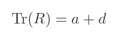
The trace of a matrix is simply the sum of all the elements on the leading diagonal. For a 2 by 2 matrix, it is given by:

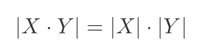
We will make use of the rule that the determinant of the product of two matrices is equal to the product of the determinants of the two matrices:

Using this rule, we can show that the determinant of S is equal to the square of the determinant of R:

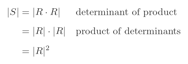
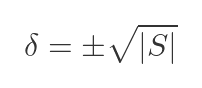
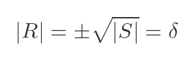
This means that, if R is the square root of S, then the determinant of R must be equal to plus or minus the square root of the determinant of S. This is the quantity we previously called δ:

Also, as a reminder, the 2 by 2 unit matrix I is equal to:

The characteristic equation

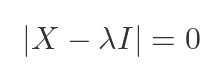
We are going to make use of the characteristic equation of R. We won't make direct use of it, but it plays a part in the Cayley–Hamilton theorem, which we will use next. The characteristic equation tells us that λ is an eigenvalue of the matrix X if and only if:

We can substitute the known values for R and I into the general equation:

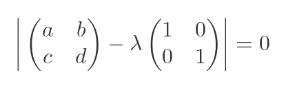
Then we can add the two matrices to simplify the determinant:

We can then expand the 2 by 2 determinant:

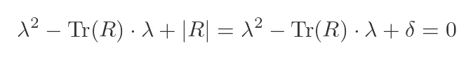
Simplifying the terms gives:

Now we know from earlier the (a + d) is equal to Tr(R), and also that (ad - bc) is equal to |R| which in turn is equal to δ. This gives us a quadratic equation in λ:

We could solve this equation to find the eigenvalues, but we aren't going to do that here. Instead, we are going to use the Cayley-Hamilton theorem.

The Cayley-Hamilton theorem

We won't look at the Cayley-Hamilton theorem in detail here, but it can be summarised as follows: every square matrix satisfies its own characteristic equation.

What does this mean? Well, if a matrix M has a characteristic equation of the form:

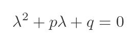
Then Cayley-Hamilton says that if we replace λ with M, the equation will still be satisfied:

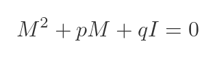
There is a small wrinkle here. λ is a scalar, so the original characteristic equation is a scalar equation. But M is a matrix, so we need to use a matrix equation. We can't add the scalar p to the other matrix terms. The theorem requires us to first multiply p by the unit matrix, as shown.

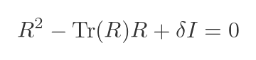
We can apply this to our matrix R. Substituting our previous values into the equation:

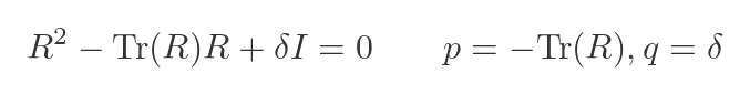
Finding R in terms of S

Our solution is now closer than it might look. We aim to find R, the square root, for any given S. The problem is that our equations currently contain only terms in R. But R and S are related. If we could express some of those terms using S instead, we might be able to solve for R.

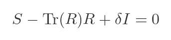
There is one thing we can do straight away. The previous equation had a term in R squared, and of course we know that is equal to S:

The next obvious term to look at is Tr(R). Can we convert this to something else, perhaps something involving Tr(S)? We know from earlier that Tr(R) is a + d. Can we find a similar expression for Tr(S)? Well we know that S is R squared, so we can find S in terms of the values a to d by matrix multiplication:

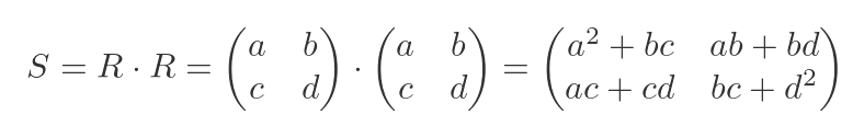
Tr(S) is just the sum of the two terms in the leading diagonal:

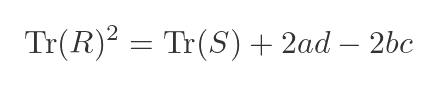
Now the a² and d² are quite interesting. We know that Tr(R) is a + d, so squaring that will give us quite a similar expression:

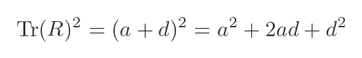
Comparing the previous expressions gives the following relationship between Tr(R) and Tr(S):

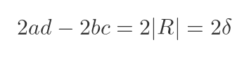
But, of course, ad - bc is the determinant of R. And we already know that the values of |R| for the solutions of the C-H equation are our old friend δ, in its positive and negative forms:

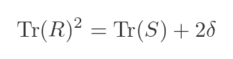
Putting this back into the previous equation gives:

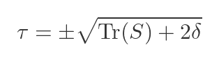
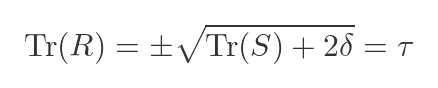
We can now take the square root to find Tr(R). Once again, we must consider the positive and negative cases. This turns out to be the value 𝜏 that we defined right at the start:

Finding the solution

If we go back to our previous solution to the C-H equation using R:

Making the substitutions for R² and Tr(R):

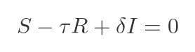
This can be easily rearranged to prove the square root formula:

An example

Let's verify this with an example. We will find the root of the following matrix:

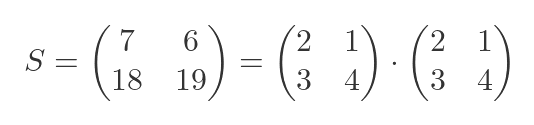
The matrix has been deliberately chosen as the square of a reasonably simple matrix, so we don't have to deal with messy radicals when we calculate R. But it isn't a trivial case, so it is a fair test.

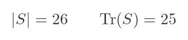
We can find the trace and determinant of S. We won't go through this in detail, it can ce easily verified using an online matrix calculator:

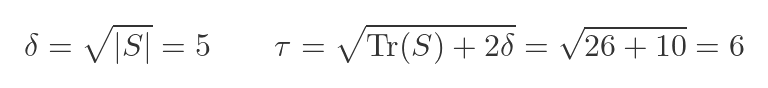
We can then calculate the positive values of δ and 𝜏:

Putting these values into the square root formula gives:

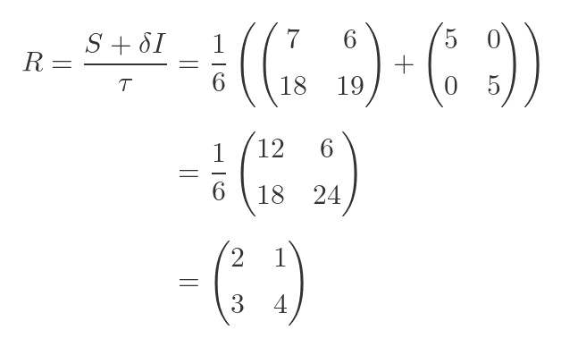
This is the value of R we used to create S, so we know it is the correct square root.

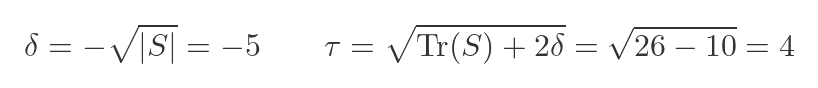
What if we choose the negative value of δ? This will also affect the value of 𝜏:

Performing the same calculation as before, we get:

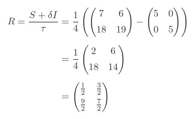
This is a different matrix, but if we square it, we get the same result, S.

We must also consider the negative values of 𝜏. It can be -6 when δ is 5, or -4 when δ is -5. Since 𝜏 only appears as the denominator, changing its sign effectively negates the whole matrix. So S has 4 square roots, the two given above and their negatives.

Related articles

• What is a matrix?
• Determinants
• Matrix inverse
• 2D transformation matrices
• Combining and inverting transform matrices
• Solving simultaneous equations with matrices
• Introduction to eigenvectors
• Diagonalising matrices