Diagonalising matrices

A diagonal matrix is a square matrix where every element except the leading diagonal is zero.

Since most of the elements are zero, certain calculations on the matrix are a lot easier than a general matrix. For example, the determinant of a large, general matrix involves a large number of multiplications, but the determinant of a diagonal matrix is simply the product of the diagonal elements.

Of course, most matrices are not diagonal. However the process of diagonalisation often allows us to find a diagonal matrix that shares some of the properties of the original matrix. We can then perform calculations a lot more easily on the diagonal matrix. The results can then be applied back to the original matrix.

We say that the diagonalised matrix is similar to the original matrix (a term that we will define below), which allows certain calculations to be shared by both matrices.

In this article, we will look at the properties of diagonal matrices, and define what we mean by similar and diagonalised matrices. We will then look at several practical methods of diagonalising a matrix.

Diagonal matrices

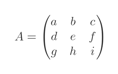
Here is a general matrix. We will use a three-by-three matrix as an example:

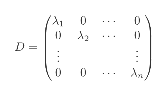
A diagonal matrix has the form:

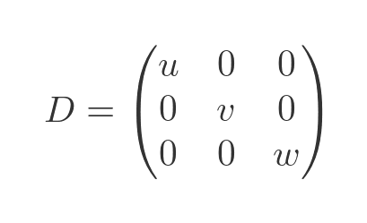
In the diagonal matrix, every term not on the leading diagonal is zero.

Diagonal matrix multiplication

Many operations are greatly simplified for a diagonal matrix compared to a general matrix. Let's start with matrix multiplication. Here is the product of two general matrices:

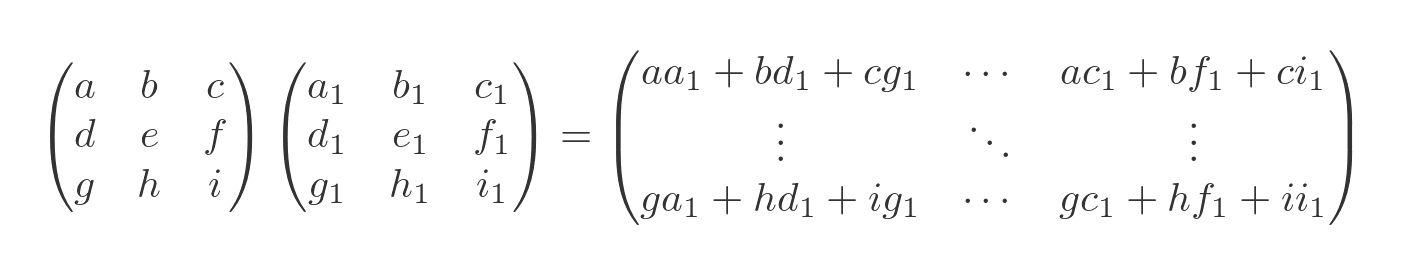
Each term in the result is the sum of the products of two values from the original matrices. The number of terms increases factorially as the size of the matrix grows. In other words, it gets very big very quickly.

For a diagonal matrix, all the terms except for a, e and i are zero, so all the products that involve any other terms will go to zero. We won't go through it in detail here, but it is easy enough to verify that the only remaining terms are on the diagonal. Applying this to the product of two diagonal matrices gives:

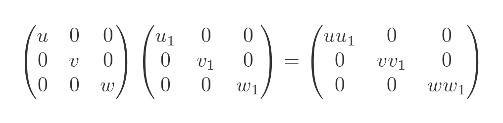
This is much simpler than the general expression. And, for larger matrices, the additional number of calculations just grows linearly (a four-by-four matrix only has four non-zero terms, and so on).

It is sometimes useful to calculate the integer power of a matrix. This works similarly to the power of a number. The square of a matrix is the matrix multiplied by itself, the cube of a matrix is the matrix multiplied by itself twice, etc.

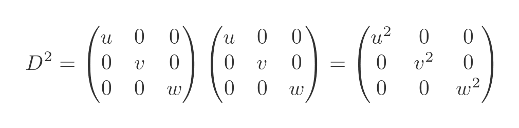
For a general matrix, the easiest way to find the nth power is by repeated matrix multiplications. But for a diagonal matrix, there is a much quicker way. Using the multiplication result from before, we can see that the square is found by squaring the diagonal elements:

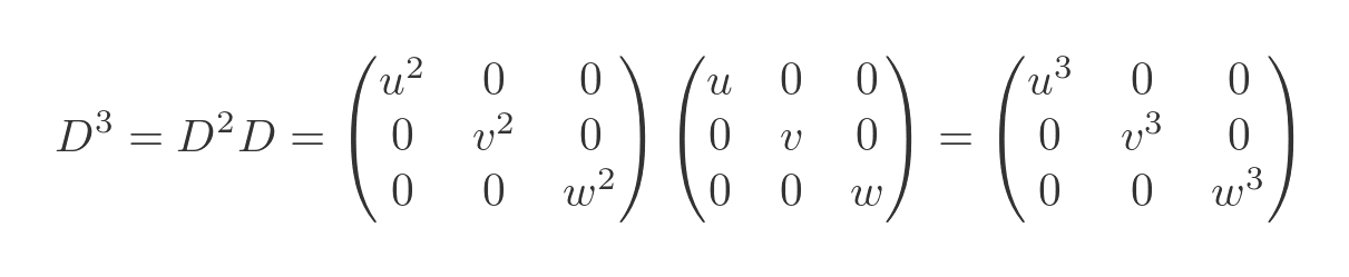
To find the cube of the matrix we can multiply the square by the matrix:

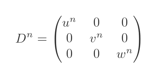
This can be extended to any power of n:

Diagonal matrix determinant and inverse

The determinant of a three-by-three matrix is given by:

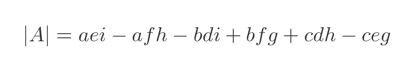
As is the case with multiplication, the complexity of the determinant increases as the factorial of the matrix size. But as before, with a diagonal matrix, we can eliminate any terms in the determinant that contain anything other than a, e and i, because all the other elements are zero. So we are only left with the first term. For our diagonal matrix, this reduces to:

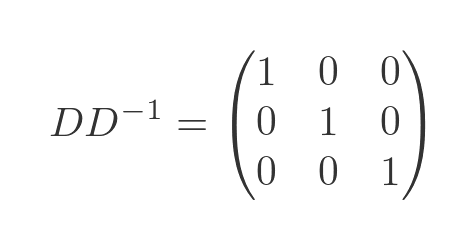
Finding the inverse of matrix requires the determinant and the matrix of cofactors (which also becomes complex for large matrices). The inverse of a diagonal matrix is much easier. We need to find the inverse matrix such that:

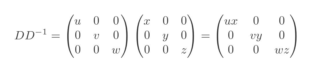
We won't prove it here, but it is easy to show that the inverse matrix also has to be diagonal. Assuming it has diagonal elements x, y and z, we have:

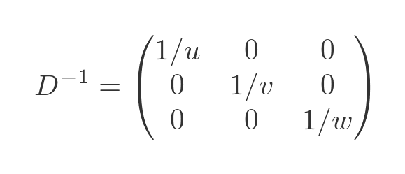
This tells us that x = 1/u, y = 1/v and z = 1/w so the inverse matrix is:

Other calculations, such as calculating the eigenvalues are greatly simplified.

Similar matrices

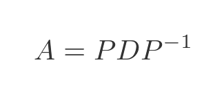
Two square matrices, A and D, are said to be similar if there is a matrix P such that:

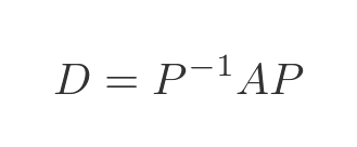
There is also an inverse relationship that relates A to D:

We often use this idea when dealing with combined transform matrices. For example, consider this matrix:

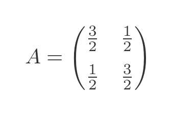
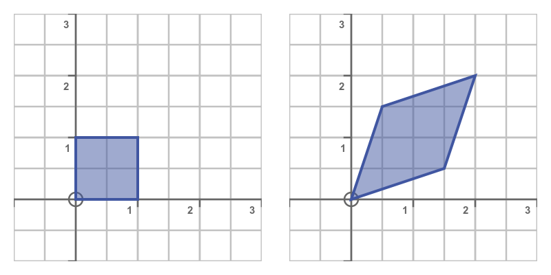
If you are familiar with matrix transforms, you might recognise this as a shear transformation. If we take a square, with four corners at (0, 0), (0, 1), (1, 1) and (1, 0), we can transform the square by multiplying each of its corners by the matrix A. This transforms the shape, as shown here:

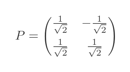
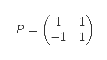
This matrix has been carefully chosen as an example, and I happen to know a value of P that will give a nice result:

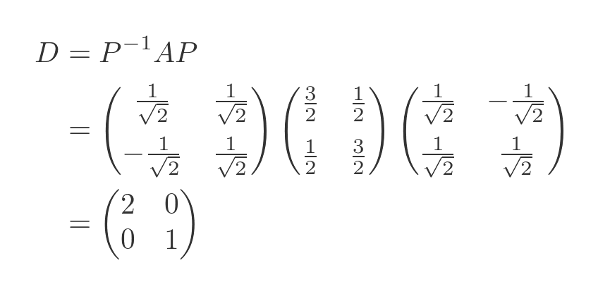
So we can use the equation above to find a value fo D that is similar to A. It also happens to be a simple, diagonal matrix:

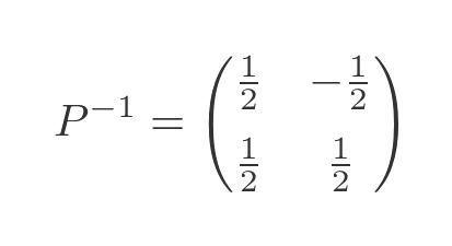
Applying the inverse function gives us A in terms of D and P:

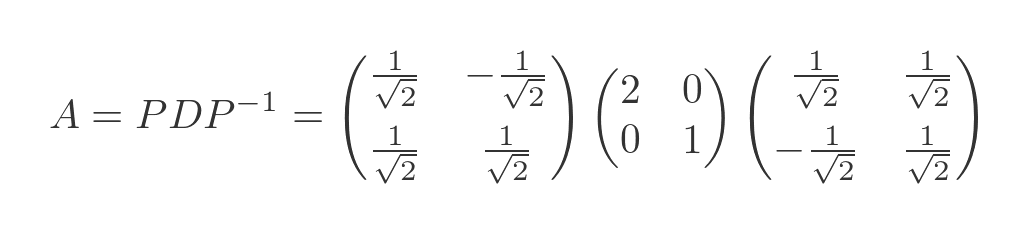
It is interesting to look at the three matrices as individual matrix transformations. What we have done, in effect, is to separate the transform matrix A into three simpler transforms. Matrix transformations are applied in reverse order so we have:

• The last matrix, the inverse of P, is a rotation matrix. It rotates the object by 45 degrees clockwise.
• The second matrix, D, is a scaling matrix. It scales the object by 2 in the x-direction, and by 1 in the y-direction - in other words, it stretches the shape by a factor of 2 in the x-direction only.
• The first matrix P, rotates the shape by 45 degrees in the counterclockwise direction.

Here are the three stages, applied one after the other:

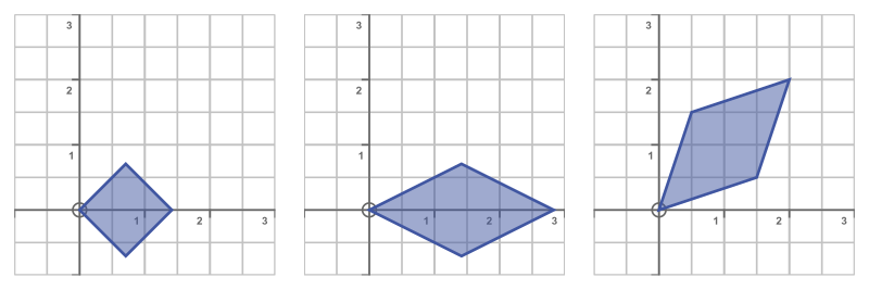
The LHS shows just the initial rotation, the middle image is the rotation plus x-scaling, and the RHS is all three transforms.

One way to understand this is that the first transform changes the frame of reference, the second transform does the actual transformation, and the final transform changes the frame of reference back to the original.

When we say that A and D are similar, one way to interpret that is that they both represent the same transformation, but defined in a different frame of reference.

Determinant of the transform

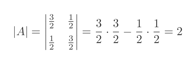
While it is not proof, we can gain a bit more confidence the A and D represent equivalent transforms by looking at the determinants. The determinant of a 2-dimensional transform matrix has a useful geometric interpretation - it is equal to the area scale factor of the transform. In our case, the unit square (with an area of 1) is transformed into an equilateral trapezium with diagonals of length 2 and 1 (therefore an area of 2). The transform doubles the area of the shape. We would therefore expect A to have a determinant of 2, which it does:

But if D represents the same transform in a different frame of reference, then we would expect its determinant to also be 2. Which it is:

What similarities do similar matrices have?

We have seen that similar matrices have the same determinant, but it doesn't end there. They have the same characteristic equation. This means that they have the same eigenvalues and the same trace, as well as the same determinant because these properties can all be derived from the characteristic equation.

Similar matrices do not have the same eigenvectors, but their eigenvectors are related. They have the same number of eigenvectors, and the eigenvectors are related by the matrix P. If v is an eigenvector of A, the P times v will be an eigenvector of D.

Finally, although in our example here one of the similar matrices is diagonal, that is not a requirement. Two non-diagonal matrices can be similar.

Eigevectors and eigenvalues

Eigenvectors and eigenvalues are described more fully in this article. We will give a summary here, as this will be useful in the discussion that follows.

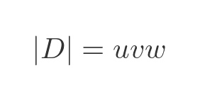
If we take a particular matrix square M and multiply it by a vector v the result will be a vector w.

In many cases, the vector w will be completely different to v. It will point in a different direction and have a different length.

However, there may be certain values of v for which the result w will point in the same direction as v. Those values of v are called eigenvectors. Each matrix M will have a particular set of eigenvectors. For an n by n matrix, there can be up to n eigenvectors (there might be fewer, or none at all).

For each eigenvector v, the corresponding w will point in the same direction but might be a different length. If the length of w is equal to the length of v multiplied by some factor λ, we say that λ is the eigenvalue of v. If the eigenvalue is negative, then w will still be parallel to v point in the opposite direction.

Diagonalisation using the eigenvectors and eigenvalues

A simple way to diagonalise a matrix is based on the eigenvectors and eigenvalues. This works well for smaller matrices where it is relatively easy to find the eigenvectors and eigenvalues. For larger matrices, where this becomes very difficult, there are other techniques. There are also numerical techniques for finding an approximate diagonal matrix.

We won't prove the results here, or cover the alternative techniques here. These will probably be a future article.

Our n by n matrix, A, has the following n eigenvectors, where each eigenvector is a vector of length n:

Diagonalisation is only possible if A has n independent eigenvectors. Some matrices do not meet this condition, and such matrices cannot be diagonalised. Assuming A meets this condition, it will also have the following n eigenvalues:

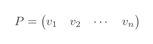
It can be shown that the matrix P is a square matrix formed from all the eigenvectors, where each eigenvector forms one column of the matrix. This is sometimes called the modal matrix for A:

It can also be shown that the matrix D will be a diagonal matrix where each diagonal element is one of the eigenvalues:

Of course, the eigenvalues and eigenvectors don't have any particular natural order. We have labelled them 1 to n in some arbitrary order. However, each eigenvector is associated with a specific eigenvalue. We can create P using the eigenvectors in any order we wish, but we must then create D using the eigenvalues in the same order. In other words, v1 and λ1 must correspond, and so on.

Example with 2 by 2 matrix

So now let's diagonalise A by finding its eigenvectors and eigenvalues. The result should give us D and P.

The article mentioned above gives a detailed description of how to find eigenvectors and eigenvalues for a matrix, so we will not show detailed working here. We will show enough steps to be able to follow if you are familiar with that article.

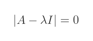
We find the eigenvalues by solving the characteristic equation:

Substituting the known values for A and I gives:

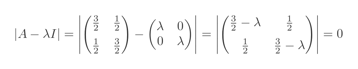
Evaluating the determinant gives:

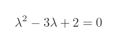
This is a quadratic equation with two solutions (the two eigenvalues):

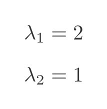
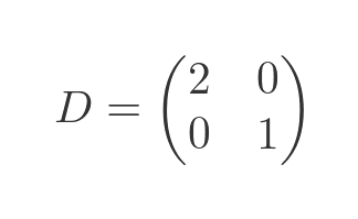
The diagonalised matrix is formed using the eigenvalues on the diagonal as we saw earlier:

As described in the linked article, the eigenvectors are solutions to this equation, for the two eigenvalues:

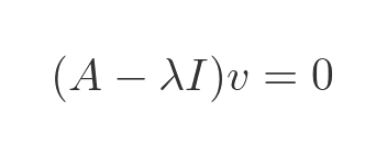
We won't go through the details but two possible solutions are:

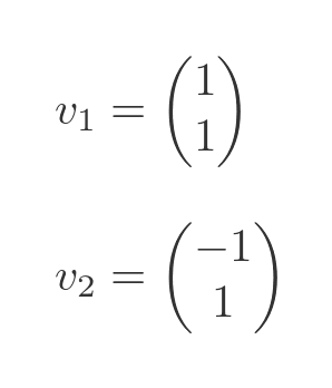
These vectors aren't the only possible solutions. If we multiply the vectors by any non-zero factor, they will still be valid solutions. It will be useful to divide them both by root 2, as we will see in a minute. So we will use these two eigenvectors:

This gives us a P value of:

The D and P values we calculated here correspond to the values we used in the transforms in the section on similar matrices above.

Why did we mess around with the P values? Well, we could have used a P value of:

Then its inverse would be:

This works perfectly well, and it still gives us exactly the same value for D. However, when we look at the geometric transforms it isn't quite as nice. This P matrix rotates the shape and also enlarges it. The inverse of P rotates the shape back and also shrinks it by the equivalent amount.

When we divide the eigenvectors by root two, we normalise them (ie the new vectors have using length). This in turn ensures that P has a determinant of one, so transforming with P produces rotation with so scaling. This is a bit cleaner, because each vector produces a separate, simple transformation.

See also

• What is a matrix?
• Determinants
• Matrix inverse
• 2D transformation matrices
• Combining and inverting transform matrices
• Solving simultaneous equations with matrices
• Introduction to eigenvectors