Differentiation - the quotient rule

The quotient rule allows us to find the derivative of the quotient of 2 functions. It has similarities with the product rule, and it may be worth studying the product rule before the tackling quotient rule if you haven't already done so.

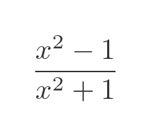
Here is an example of the sort of function we can differentiate, the quotient of 2 quadratic functions:

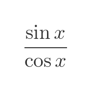
Here is another example, the quotient of 2 trig functions. This function is, of course, equal to tan(x):

In this article, we will give some worked examples of the rule. In some of the cases, we will also show how the same result can be obtained by differentiation from first principles. We will then look at an informal geometric interpretation of the formula, before showing a proof of the technique.

The rule

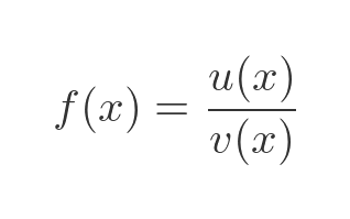
The quotient rule applies to functions of this form:

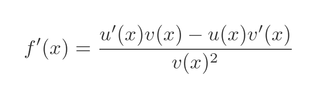
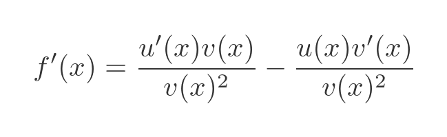
The first derivative can be calculated as:

Example - quotient of two quadratics

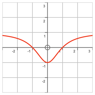
We will illustrate the technique using this function from earlier:

Here is a graph of the function:

This function has the form of a quotient:

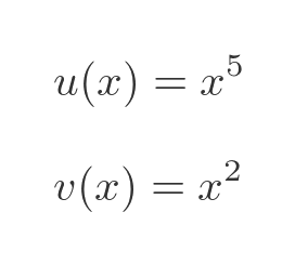
Where:

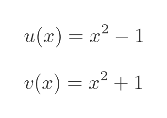
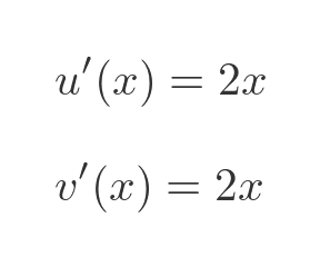
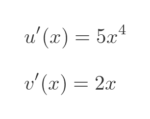
We will need the first derivatives of u and v. These are both simple polynomial functions, so we can differentiate them in the normal way:

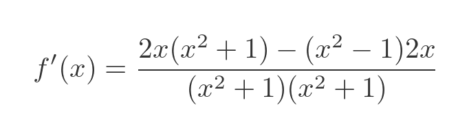
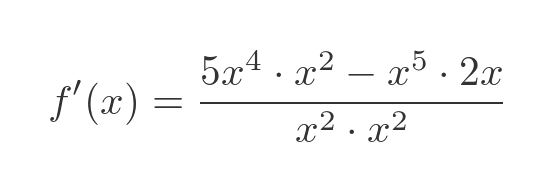
Now we need to plug these equations into the quotient rule formula:

Substituting u, v and their derivatives gives:

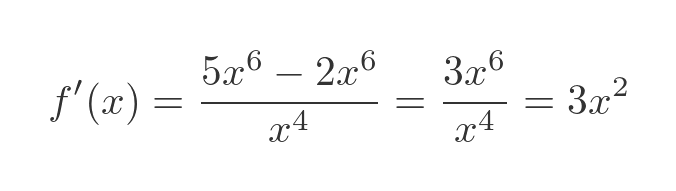
Multiplying out the top and bottom expressions gives:

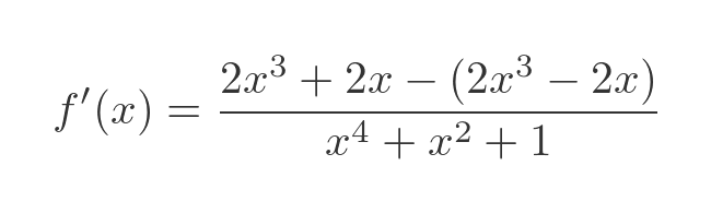
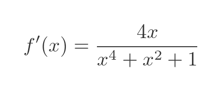
The terms in x-cubed on the top line cancel out, so the derivative simplifies to:

As a final check, let's look at the graph of this function. This shows f in red and f' in cyan:

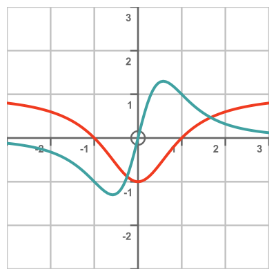
This looks quite plausible:

• The slope is 0 when x= = 0.
• The slope is negative when x < 0 and positive when x > 0.
• The slope is steepest at around x = 0.6 and x = -0.6.
• The slope tends to 0 when x gets large in the +ve or -ve directions.

Example - quotient of sine and cosine

As a second illustration, we will use this function from earlier:

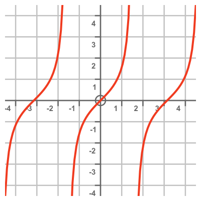
Here is a graph of the function. As we noted earlier, this is simply the tan function:

This function also has the form of a quotient:

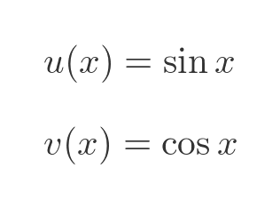
This time, u and v are:

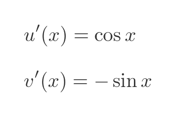
The derivatives of sine and cosine are standard results:

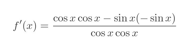
Plugging these into the quotient rule formula gives:

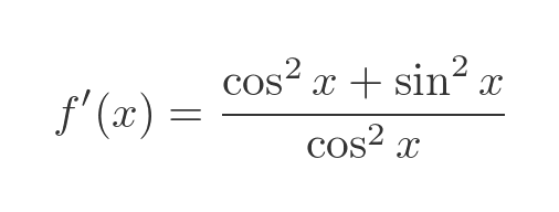
This simplifies to:

We can apply the Pythagorean identity, cos squared plus sin squared equals 1, to get this:

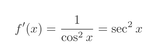
The derivative of tan is a standard result, so we already know this equation is correct. For completeness, here is a graph of tan (red) and its derivative sec squared (cyan):

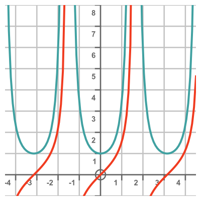
This again looks plausible. It is always positive (because the tan graph always increases), it has a minimum value of 1 when x is a multiple of π, and it zooms off to positive infinity when x is an odd multiple of π/2.

Verifying the formula

We can verify the formula by applying it to a case where we already know the correct result. We have already done this with the tan function, and we found that applying the quotient rule to sin over cos gave the standard result for differentiating tan directly.

But for good measure let's try again using this function:

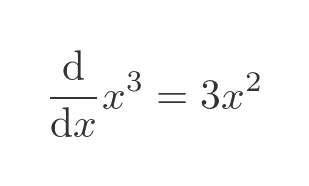
Of course, the function can be reduced to x cubed, so we know the result we are expecting:

Let's apply the quotient rule to the original expression. Here are u and v:

And here are their derivatives:

This is the resulting quotient rule formula:

We can simplify this. And of course, it gives the same result as differentiating x cubed directly:

Geometric interpretation of the quotient rule

The geometric interpretation of the quotient rule has a similar form to the geometric interpretation of the product rule, but with a couple of extra steps. It may be worth familiarising yourself with the product rule interpretation if you haven't already seen it.

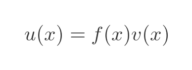
We know that f(x) is the quotient of 2 functions u(x) and v(x):

This can be rearranged as:

This allows us to represent the value of u(x) as the area of a rectangle with sides f(x) and v(x). This is shown on the left here:

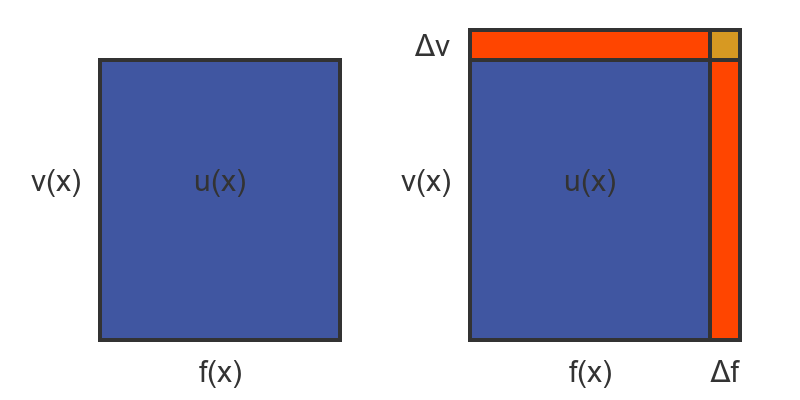
Now let's suppose we increment x by a small amount Δx. This caused f to change by a small amount Δf and v to change by a small amount Δv. That is shown on the right, above.

Incrementing x adds two orange rectangles to the area. The right-hand rectangle has area Δf by v, and the top rectangle has f by Δv.

There is also a tiny yellow rectangle size Δf by Δv. As Δx gets very small, this rectangle gets smaller much more quickly than the two orange rectangles, so we will ignore it in our calculations.

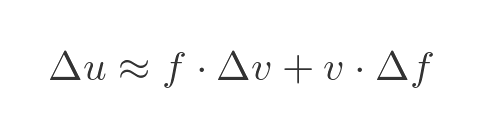
So the approximate change in u as we change x by Δx is given by the orange region:

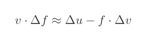
We will rearrange this to bring the term in Δf to the left, as ultimately we want to solve for f':

Now let's multiply through by v:

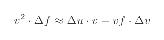
Now we can make use of the fact that vf = u, to eliminate f from the RHS:

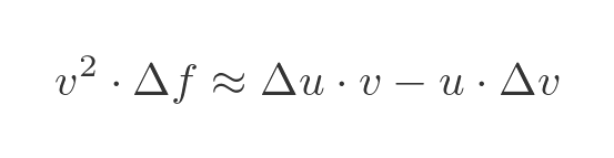
Dividing through by Δx we find the relationship between the approximate rates of change:

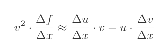
Dividing through by v squared gives and approximate expression for the rate of change of f:

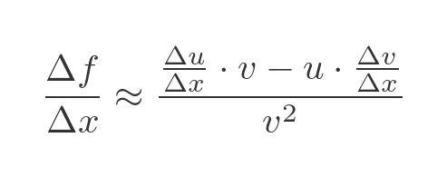
As Δx tends to 0 this resembles the quotient rule formula:

Proof of the quotient rule

There are several proofs of the quotient rule, but probably the most straightforward is this proof using the product rule in conjunction with the chain rule. The proof below assumes you already know those two rules.

There are 2 steps to the proof. First, we will convert the quotient function into a product of two functions, where one of those functions is a composed function - that is, one function applied to the result of another, such as r(v(x)). In the second part of the proof we simply apply the product rule and chain rule in the usual way.

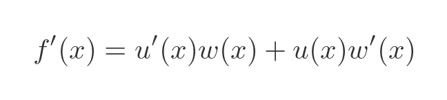
We can write the quotient function as a product, like this:

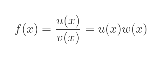
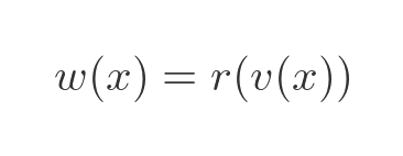
For this to work, the function w must be equivalent to the reciprocal of function v. In other words w is:

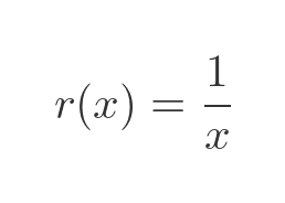
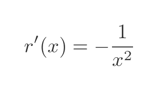
Where r is the reciprocal function:

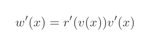
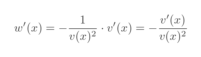
We now have the quotient equation in a form that we can differentiate using the product rule and chain rule. We are going to need the derivative of w later, so let's find it now, using the chain rule applied to r(v(x)):

We can find the derivative of r, since r is 1/x which has a standard derivative:

Applying this to w' gives us an expression that depends only on v and v':

Now we can use the product rule to find f':

Substituting the known values of w and w' gives us:

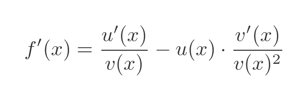
Finally, we can multiply the first term on the RHS by v(x)/v(x) so that the terms have a common denominator:

This gives us the quotient rule:

See also

• Slope of a curve
• Differentiation from first principles - x²
• Differentiation from first principles - a to the power x
• Second derivative and sketching curves
• Differentiation - the product rule
• Differentiation - the chain rule
• Derivative of sine, geometric proof
• Differentiation - L'Hôpital's rule