Second derivative and sketching curves

In this article, we will look at the second derivative of a function. This is sometimes called the second order derivative.

What is the second derivative?

To find the second derivative of a function, we simply differentiate the function in the usual way, and then we take the result and differentiate it again. In other words, we differentiate the function twice. Here is an example function:

Using Leibniz's notation, the first derivative is calculated using the nth power of x rule in the normal way:

To calculate the second derivative we just differentiate again:

Notice the notation. The double differentiation is indicated by adding a 2 to the top and bottom of the d/dx.

We sometimes use the alternative, Lagrange's notation, for derivatives. In that case, we write the original function as f:

We write the first derivative as f prime:

We write the second derivative as f double prime:

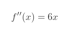
The two notations are interchangeable, but sometimes one or the other is a slightly more suitable way to express the equation.

Sketching graphs - stationary points

It is often useful to be able to sketch a graph of a function. We do this by identifying a few key points of the graph and making a rough estimate of the curve. This gives us a good idea of the type of curve we are dealing with.

To some extent, modern inventions such as graphing calculators, or plotting software (such as generativepy that I use for creating articles like this), make sketching slightly less useful. But we still need to know which region of the graph to plot, otherwise we might miss important features.

Stationary points - that is local minimum and maximum values - are useful points on a graph that can often be found quite easily. They are simply points where the derivative of the function is 0. We use the second derivative to classify the stationary point as a minimum or maximum value.

In addition to stationary points, we can also try to find roots (the points where the curve crosses the x-axis), and asymptotes (the behaviour of the curve as x tends to +/- infinity).

Example - local minimum

As a first example, let's look at the equation:

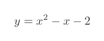
We can also find the first and second derivatives, using the standard rules of differentiation for powers of x

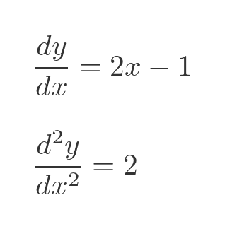
The turning points of the graph are the points where the first derivative of the curve is 0. Looking at the equation for the first derivative, it is 0 when x is 0.5. This means that the curve has a gradient of 0 at that point, in other words, the tangent to the curve is horizontal.

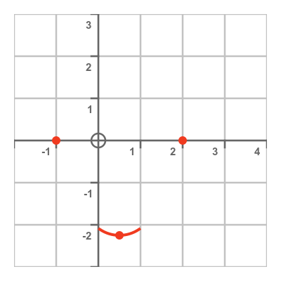
From the original equation for y, we can calculate that when x is 0.5, y -2.25. So we know that the curve passes through point (0.5, -2.25), which we will call P, and has a horizontal tangent at the point. We can show this information on a graph like this:

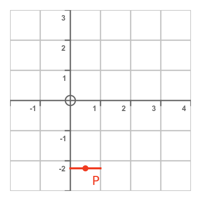
We know that the curve touches the point with a horizontal tangent, but we don't know exactly how. This is where the second derivative is useful. Remember, the second derivative tells us the rate of change of the rate of change of the curve. In other words, it tells us the rate of change of the slope.

We saw above that the second derivative of this curve is 2, which means that the slope of the curve is always increasing.

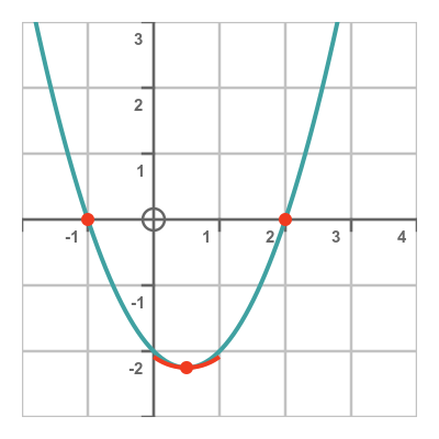
Since the curve has a slope of 0 at P, and the slope is increasing, it follows that the slope must be negative to the left of P, and positive to the right of P. This means that the value of the curve at P must be smaller than the value of the curve on either side of it. So P is a local minimum value. We can show this on the graph using a U-shaped curve around P:

As mentioned earlier, we can also find the roots of the equation (the points where the curve crosses the x-axis) to help sketch the curve. Since the original curve is quadratic, we can use the quadratic formula to find these roots. These turn out to be -1 and 2, and we have marked the points (-1, 0) and (2, 0) on the axes above.

Finally, we can also consider the asymptotes. As x gets very large, the x squared term grows faster than the other terms, so that term dominates the shape of the curve. This means that the curve tends to towards infinity as x tends towards positive infinity. And since x squared is always positive, it also means that the curve tends towards infinity as x tends towards negative infinity.

Putting these three facts together, we can sketch the curve like this:

We could simply have drawn this curve using graph plotting software. What the sketch told us, though, is that the curve does something interesting when x is -1, .5, and 2. Once we go much outside that range, the curve doesn't do anything remarkable, it just makes the monotonous journey to infinity. So it tells us which part of the graph is worth plotting.

Example - local maximum

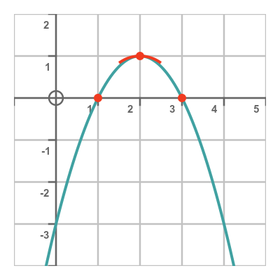
Here is a second example:

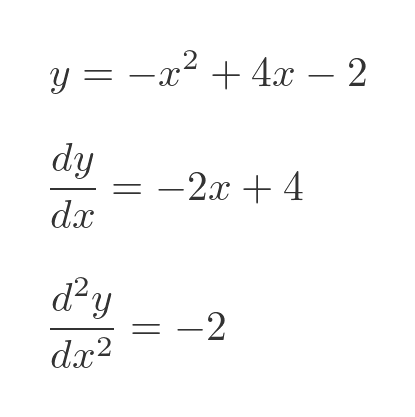
This time the first derivative is zero when x is 2, which indicates that this might be a turning point. When x is 2, y is 1.

This time the second derivative of the function is -2, which means that the slope of the curve is always decreasing.

Since the curve has a slope of 0 at P, and the slope is decreasing, it follows that the slope must be positive to the left of P, and negative to the right of P. This means that the value of the curve at P must be greater than the value of the curve on either side of it. So P is a local maximum value. We show this on the graph using an inverted U-shaped curve around P:

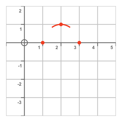
If we solve the quadratic equation, this time it has roots at 1 and 3. These points are also marked on the plot above.

This time, since the x squared term is negative, the curve tends to negative infinity as x tends to either positive or negative infinity

Here is a sketch of the new curve. This time it curves downwards:

Example - points of inflection

There is a third situation where the rate of change of a curve might be zero at a certain point. A point of inflection occurs when a curve is initially increasing, then goes flat, and then starts increasing again. There is an equivalent situation for the case of a decreasing curve.

At a point of infection, the second derivative is always zero. However, the second derivative being zero doesn't guarantee that it will be a point of inflection. It is a necessary but not sufficient condition. Sometimes local minima or maxima have second derivatives of zero. The only way to be sure is to check the value of the curve on either side of the point of interest.

We will look at this equation:

It will be useful to know that the curve and its first derivative can be factorised like this:

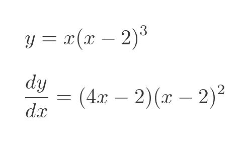
So what can we say about this curve? The first derivative is 0 when x is either 0.5 or 2 (we can tell this from the factorised first derivative).

When x is 0.5, the second derivative is positive (it evaluates to 9) so that point is a local minimum. When x is 2, the second derivative is zero so we don't know what sort of stationary point it is.

Looking at the factorised main function, we can see that the function has roots at 0 and 2 (the second root is coincident with the second stationary point). So the important points on the graph look like this:

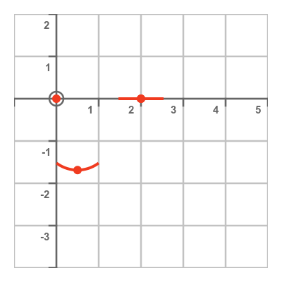
This is a fourth-degree polynomial (it has a term in x to the power 4), and all even powers of x tend towards positive infinity as x tends towards either positive to negative infinity. This allows us to sketch the curve like this:

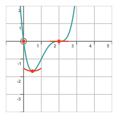
We know that the stationary point at 2 must be a point of inflection, because to the left the curve is increasing from the local minimum at 0.5, and to the right, the curve is increasing towards infinity. There are no other stationary points, so this is the only type of stationary point that fits.

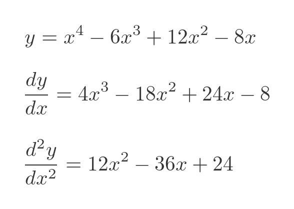
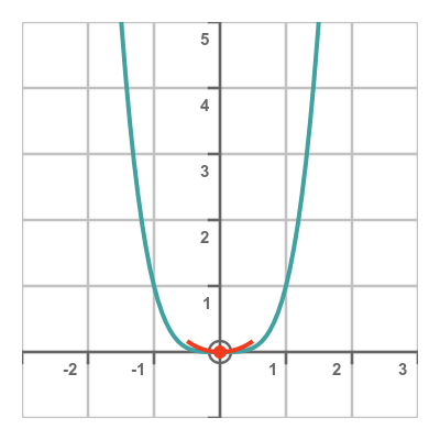
Finally, we will look at a quick example of a second derivative of zero that does not indicate a point of inflection. Here is the curve of x to the power 4:

The relevant equations are:

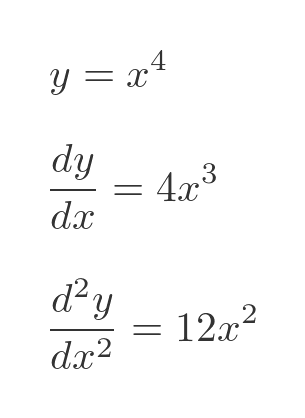
When x is zero, the first derivative is zero (indicating a stationary point), and the second derivative is also zero. But this is clearly a local minimum - the function x to the power 4 is a well-known standard curve, that has a minimum at (0, 0).

In summary, a positive second derivative indicates a local minimum, a negative second derivative indicates a local maximum, but a zero second derivative doesn't tell us anything, we need more information to decide.

Second derivative in mechanics

An everyday example of this is the motion of a car. As a car travels along, the distance s changes with time. The rate of change of s with time, of course, is the velocity of the car. The rate of change of velocity is the acceleration.

This means that the acceleration of the car is equal to the rate of change of the rate of change of the distance.

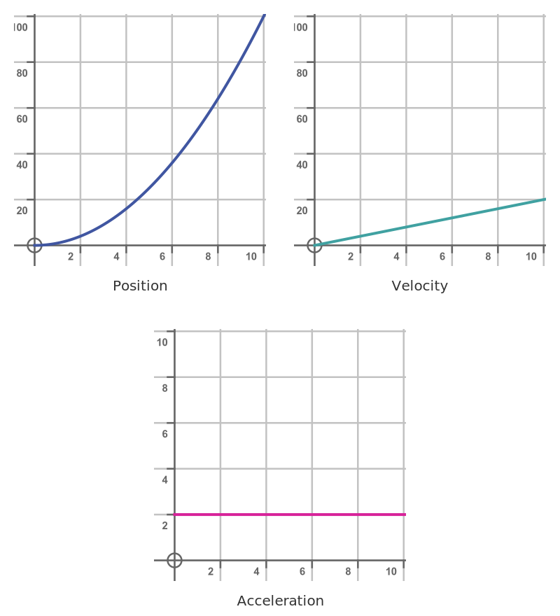
Imagine a car travelling along a straight, flat road, starting at position 0. We are told that, at time t, the car's distance from 0 is given by s where:

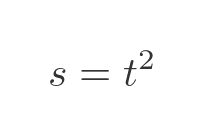
The velocity of the car, v, is the rate of change of s. It can be found by differentiating s,like this:

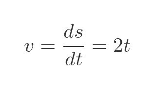
We can find the acceleration by differentiating again. This time we get a constant value:

Here are graphs of the distance, velocity, and acceleration of the car over the first 10 seconds of its motion:

Acceleration and force

According to Newton's second law of motion, the force acting on an object is equal to its mass times its acceleration.

That law allows us to relate a force to the motion of a body. In the example above, it tells us that, if the distance travelled by the car increases as the square of t, the acceleration must be constant, and therefore the force acting on the car must also be constant.

Third derivative

The third derivative of distance is equal to the rate of change of acceleration.

When the car is accelerating at a constant rate, you might feel yourself pushed back into your seat, but the force will be constant so it will feel smooth.

If the driver was to suddenly apply the brakes, the acceleration would change abruptly. A rapid change in acceleration is very noticeable.

The rate of change of acceleration is called jerk or sometimes jolt. Jerk is the rate of change of acceleration in the same sense that acceleration is the rate of change of velocity.

See also

• Slope of a curve
• Differentiation from first principles - x²
• Differentiation from first principles - a to the power x
• Differentiation - the product rule
• Differentiation - the quotient rule
• Differentiation - the chain rule
• Derivative of sine, geometric proof
• Differentiation - L'Hôpital's rule