Complex powers and roots of complex numbers

In earlier articles, we looked at the powers of a number, from simple integer powers of real numbers to more complex cases like the imaginary number i raised to the power i. In this article, we will generalise this to find z raised to the power w where z and w are both general complex numbers.

First, we will quickly summarise what we learned from the previous articles.

Real numbers

We know that a real number a raised to a positive integer power n is equal to 1 multiplied by a, n times:

We also know several other rules that apply to integer exponents n and m:

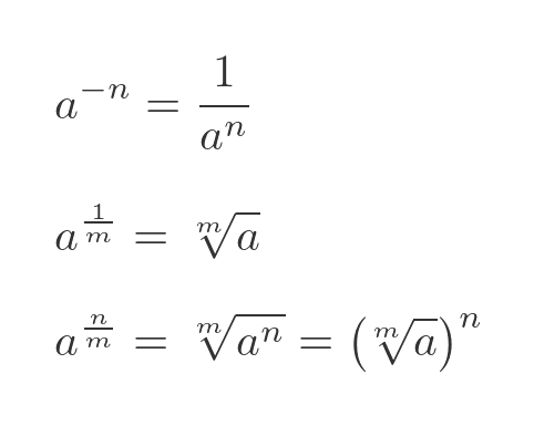
We also know that when m is even, there are 2 roots of a, one positive and one negative.

We know how to raise a to an irrational power q. If we use the Maclaurin expansion for the exponential function, we can find e to the power q and use the standard equation for changing bases to give:

Complex numbers

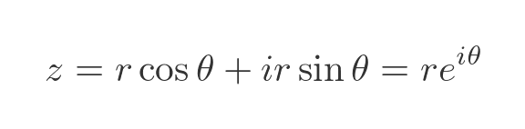
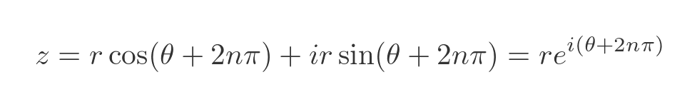
We know that a complex number can be expressed in modulus-argument form as:

We also know that this formula is cyclic. Adding any multiple of 2π to the sin and cos functions doesn't change the result, so this equation holds for any integer n:

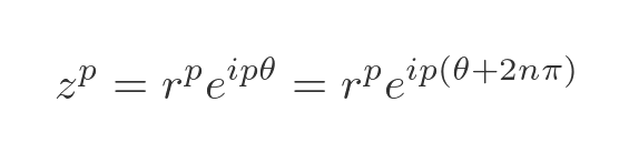
If we raise z to any real power p we get this result:

We also know that this formula can be extended for an imaginary value, p = i, to find i to the power i. Here is i in modulus-argument form:

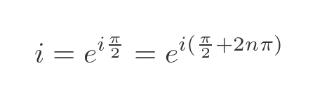
This shows the principal value and all the other values that are obtained by adding multiples of 2π to the argument. Raising the principal value to the power i gives:

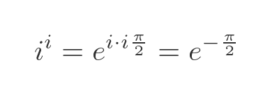
But considering all the other values gives:

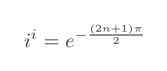
As pointed out in the linked article, since π is irrational, there are an infinite number of different solutions.

Complex number to a complex power

Now let's find z raised to the power w for 2 general complex numbers z and w:

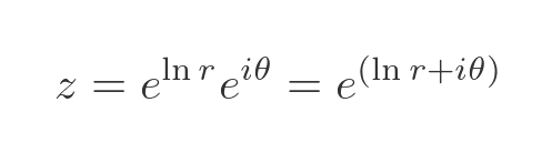
It will be useful to express z in modulus-argument form:

In the workings below, r and θ refer specifically to the values for z. We can use the result that:

To move r into the exponent, which will be useful later:

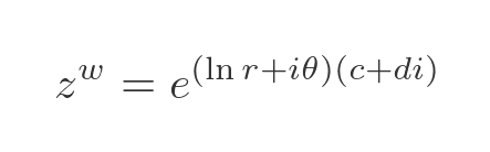
Raising this to the power w gives:

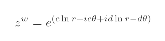
Next, we multiply out the brackets in the exponent:

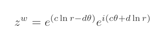
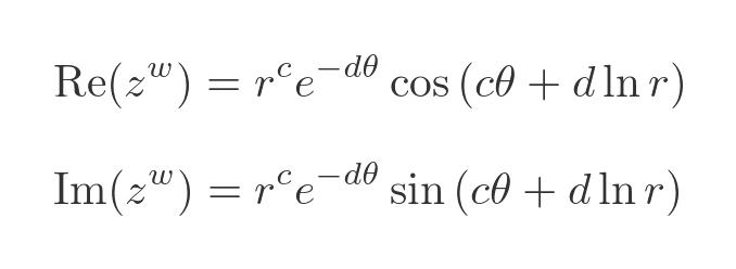
We can separate the real and imaginary parts:

The real part can be simplified. We can change the base of the first term (the exponential of c ln r) to give r to the power c:

That is the formula for z to the power w, expressed in terms of the modulus and argument of z (r and θ), and the real and imaginary parts of w (c and d). It isn't particularly pretty, but it allows us to calculate the value of the function using normal algebra.

We can use Euler's formula to find the real and imaginary parts of z:

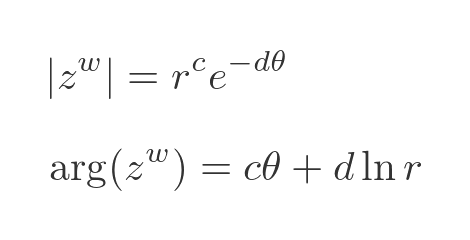
The formula above can also be expressed in modulus-argument from, like this:

Graphing the function

There are two different complex functions based on a complex number raised to a complex power.

The first is a power function:

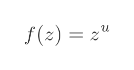
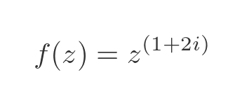
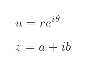
Where u is some constant complex number, for example:

The second is the exponential function:

Again where v is some constant complex number, for example:

We will look at these functions separately.

Complex power function

Here is the complex power function from before:

This is the complex equivalent of a power function such as x-squared or x-cubed in the real domain. But in the complex domain, every possible value of z yields a complex result (with a real and imaginary component).

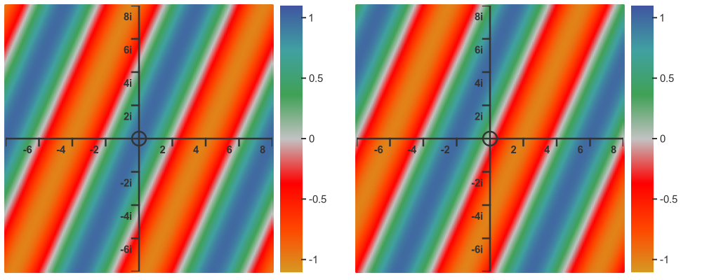
It can be difficult to represent this function as a graph, but one way to do it is like this:

Each graph represents z values as points on the complex plane. The left-hand graph shows the real part of f(z) as colours, from yellow (-10) through to blue (+10), using the scale on the right. The right-hand graph shows the imaginary part of f(z) using the same colour scale.

Here is f(z) expressed in modulus-argument form (as we saw earlier). We can substitute the values of c = 1 and d = 2 to simplify the equation:

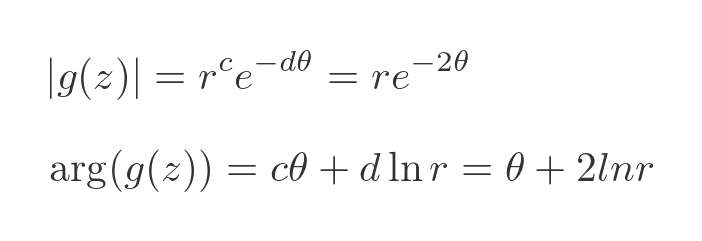
How does this relate to the graphs above? The most obvious feature of the graphs is that f(z) is very small above the real axis. This is because the modulus of f(z) is equal to the modulus of z multiplied by the exponential of -2 times the argument of z. Above the real axis, arg(z) is positive so the exponential function is less than 1, making the modulus of f(z) small.

The other main feature is that the graph is spiral in nature. This is because the argument of f(z) is equal to the argument of z plus a term in ln r. For r > 1 the log term is positive, so larger the values of of r (the modulus of z) twist the graph clockwise. For r < 1 the ln term is negative so the graph is twisted in the opposite direction.

Complex exponential functions

Here is the complex exponential function from earlier:

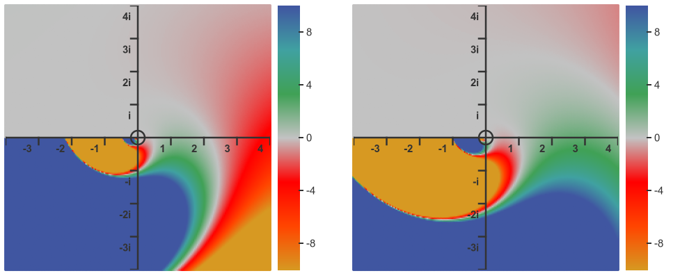
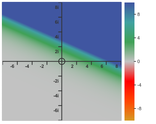
This is the complex equivalent of an exponential function (such as e to the x) in the real domain. Here is the graph for the exponential function:

Notice that the real and imaginary charts a similar but not identical. In particular, the bands aren't aligned, the imaginary bands are displaced by half the width of a band compared to the real bands (because they are based on sine and cosine terms, as we will see).

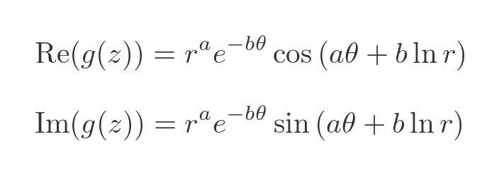
To understand this graph, we can look at the real and imaginary parts:

This formula is the same as the one we saw earlier except that this time we are using v and z in place of z and w. So in this formula, we have:

Now u is constant, so r and θ are constant. We will use these uppercase variable names for the constant terms:

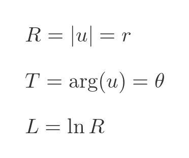
This gives the following equation for g(z) in terms of a and b (the real and imaginary parts of z).

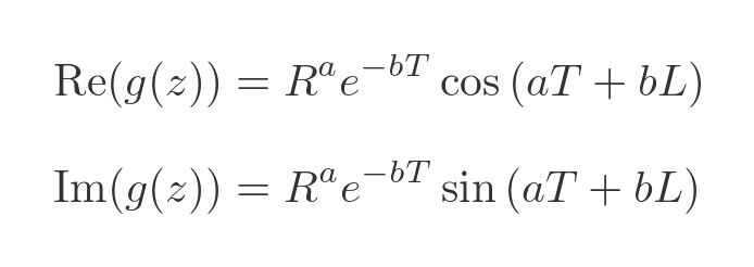
This helps us to understand the graph a little better. We can split the equations into 2 factors. First the real and imaginary cosine/sine terms:

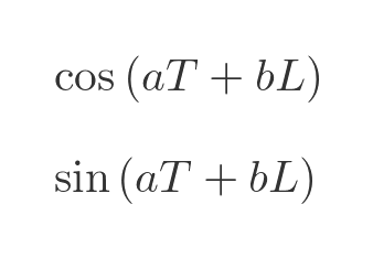
The graph for this term looks like this:

Notice that the two graphs are similar but displace relative to each other, as we noted earlier, because one is based on sine and the other on cosine. This term contributes to the banded structure of full function.

The other factor is:

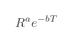
This factor is the same for the real and imaginary terms. Here is its graph:

This function is a combination of two exponential functions, with exponents of a and -bT. In this case T, which is the argument of u, happens to be negative. This means that the overall term tends to 0 when a and b are negative, which means that the bottom-left part of the graph tends to 0.

When we multiply the terms together we get the complete the graph above.

See also

• Imaginary and complex numbers
• Complex number arithmetic
• Argand diagrams
• Why does complex number multiplication cause rotation?
• Modulus-argument form of complex numbers
• i to the power i
• Euler's formula - proof
• Semiprocal numbers - z to the power i
• Complex polynomials
• Complex number trigonometry functions