Argand diagrams

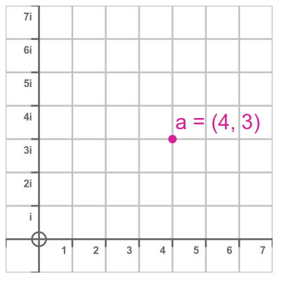
An Argand diagram is a simple way of representing the complex number plane on an (x, y) coordinate system. It uses the x-axis to represent the real part of the number, and the y-axis to represent the imaginary part. So the complex number a + bi is represented by the point (a, b) on the plane:

This might seem like an obvious idea, but it was a significant innovation at the time, and it led to a greater acceptance of imaginary numbers into mainstream mathematics. It showed complex numbers as an extension of the real number line and provides a geometric interpretation of complex number arithmetic. It also illustrated the polar interpretation of complex numbers, which explained complex multiplication and ultimately led to Euler's formula. Finally, it provided a way to visualise complex functions of complex variables.

History of imaginary numbers

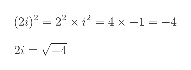
The imaginary unit i has the property that its square is -1. It is often described as the square root of -1, although the quantity -i is also a square root of -1 (in the same way that both 1 and -1 are square roots of 1). Since no real number can be the square root of a negative number, the term imaginary was coined for this new type of number.

An imaginary number is the product of i and any real number. For example 2i is an imaginary number that happens to be the square root of -4:

The problem of finding the square root of a negative number goes back a long way. In the Roman era, the Greek mathematician Hero of Alexandria (who also gave us Heron's formula) considered the problem. But at the time mathematics wasn't sufficiently advanced to offer a solution.

This issue became more important when algebraic solutions to cubic and quartic equations were discovered in the 16th century. Finding the roots of a cubic equation sometimes involved the square roots of negative numbers, even if the solutions were all real.

Solving this problem eventually led to the idea of imaginary numbers, but initially they were seen as something that only really applied to the intermediate steps in solving polynomials, and had nothing to do with real numbers.

The idea of representing complex numbers as points on a complex plane was originally suggested by Caspar Wessel in 1799 but was independently suggested again in 1806 by Jean-Robert Argand, who gave his name to the Argand diagram.

Complex number addition and subtraction

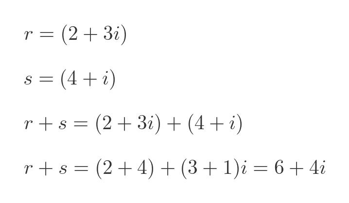
Adding and subtracting complex numbers is based on the idea that real and imaginary numbers are different things that must be kept separate. So the real and imaginary parts must be added (or subtracted) separately:

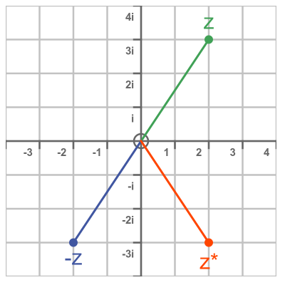
This is similar to how vector arithmetic works, and can be illustrated in a similar way on an Argand diagram:

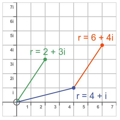
The key point here is that an Argand diagram shows that complex numbers are an extension of real numbers into two dimensions. It also gives a geometric interpretation of addition, subtraction, negation (we negate a complex number by rotating it through 180°) and the complex conjugate z^* (flipped over the real axis):

Polar form of complex numbers

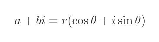
The Argand diagram can be used to represent a complex number in polar form. This works in the same way as normal polar coordinates, so the complex number a + bi can be represented as:

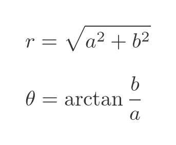
where:

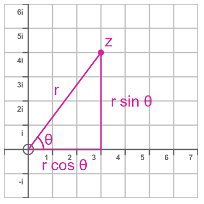
This is shown here on an Argand diagram:

The polar form of complex numbers is important because it turns out that when we multiply two complex numbers we multiply the magnitudes (r values) and add the angles (θ values). So:

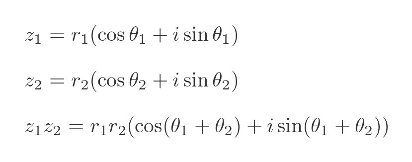
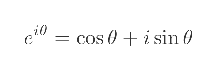
This also gives us a geometric interpretation of complex number division, powers, and roots. It ultimately leads to Euler's formula, which in turn allows us to calculate things like i to the power i:

Complex functions of complex variables

It is possible to create complex versions of various functions. For example, we can define the sin function for a complex argument z = x + iy:

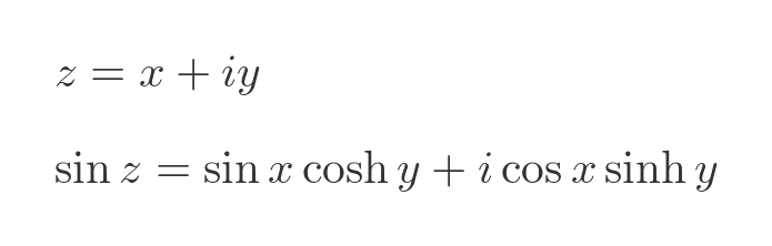
Since x and y are real values, we can calculate sin x, cosh y, etc in the usual way.

This means that for every complex value z, the complex sin function will return a complex number result. The sin function is, therefore, a 4-dimensional curve, which can be quite difficult to visualise. A standard way to do this is to plot the real and imaginary parts of the function separately:

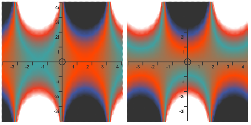
Here the left-hand image shows the value of the real part of sin z. The Argand diagram represents input values z in the complex plane. The colour of the graph at each point represents the value of the real part of sin z (ie the x value) for the value of z at that point in the plane. At this stage we aren't too interested in how the colours map onto values, we are just looking at the technique for representing values.

The right-hand image shows the imaginary part of z (the y values) in a similar way.

Summary

The Argand diagram is a useful way of representing complex number arithmetic and functions. But beyond that, it was an important step in our understanding of the many applications of complex numbers.

See also

• Imaginary and complex numbers
• Complex number arithmetic
• Why does complex number multiplication cause rotation?
• Modulus-argument form of complex numbers
• i to the power i
• Euler's formula - proof
• Complex powers and roots of complex numbers
• Semiprocal numbers - z to the power i
• Complex polynomials
• Complex number trigonometry functions