Complex polynomials

In this article, we will look at polynomials in the complex domain. This will also serve as an introduction to general functions in the complex domain.

To set the context, we will start with a very quick review of quadratic equations in the real domain.

Real quadratics

When we first learn about quadratic equations in school, we usually stick to the domain of real numbers. A quadratic equation takes the form:

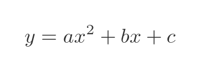
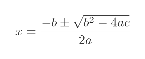
Where all the coefficients are real numbers, and x is a real variable. The solution can be found from the well-known quadratic formula:

Here is an example:

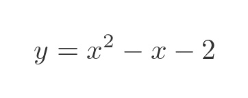
If we plot this as a graph it looks like this:

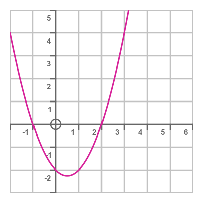
We can find the solutions either by using the quadratic formula, or for simple cases we can use the graph for guidance and factorise the equation by trial and error. Here is the factorised equation (which we can check by multiplying out the brackets to make sure it results in the original equation):

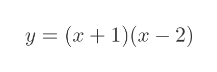
This tells us that the roots of the polynomial are -1 and 2.

Here is another example:

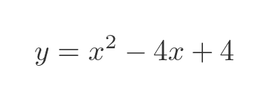
This time the graph looks like this:

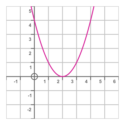
Again we can guess the factorisation:

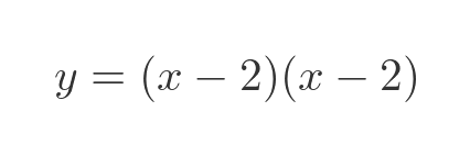
This tells us that the polynomial only has one root, value 2.

Here is a final example:

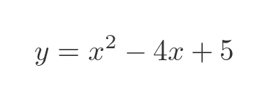
This time the graph looks like this:

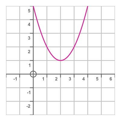
In this case, the graph doesn't cross the x-axis. We can try to use the standard quadratic formula above, substituting the values a, b, and c:

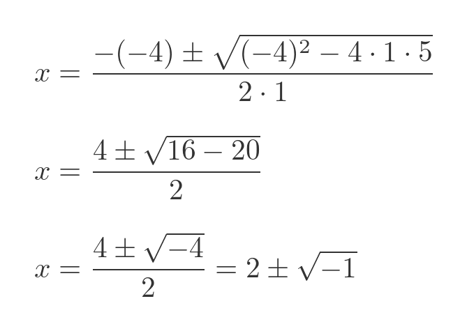
This equation requires us to find the square root of a negative number. When we first learn about quadratic equations, we are usually taught that negative numbers don't have a square root, so there is no solution to this particular quadratic equation.

A complex number solution

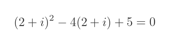
If we go slightly beyond basic high school maths, we learn that -1 does in fact have a square root, the imaginary unit, i. So we can find the solution. The quadratic goes to 0 for 2 different values of x:

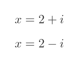
We can verify that by substituting these values into the original quadratic. It is shown here for (2 + i), we can do the same for (2 - i):

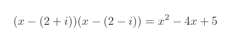
Alternatively, we can multiply out the factorised equation:

These results are easily verified using your favourite online complex number calculator.

Plotting the modulus of a quadratic

When we come to look at quadratics in the complex domain, it will be useful to look at the modulus (or absolute value) of the curve. Here is the modulus of the first case, with 2 roots:

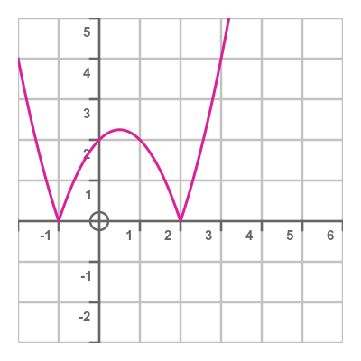
The part of the curve that would have been below the x-axis is negated so it appears above the x-axis. The roots are still in the same place, but they appear more prominent because they create points. We will see this pattern in the complex case too.

Entering the complex domain

This solution so far is a little unsatisfying. We are essentially limiting ourselves to the real domain, but then allow a complex value of x simply to solve certain equations. That gives us a tiny glimpse of another world but goes no further.

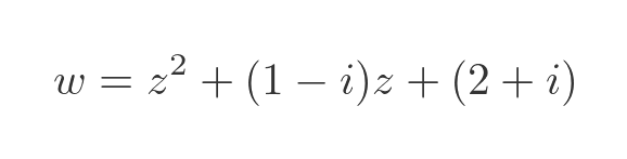
What if we allow x to take any complex value, and plot a graph of the whole thing? It is conventional to name a complex variable z, so our quadratic now looks like this:

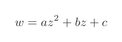
This means that the input domain of the function is the set of complex numbers. Input values can't be represented on a single axis (like x values), they need to be represented on the complex plane. We will take the equation:

Plotting the modulus of this function, as discussed earlier, results in this:

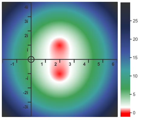
Every point on the plane represents a complex number z, the input to the quadratic. The colour of the plot at that point represents the modulus of the value of the quadratic function. The 2 red dots represent the points where the modulus goes to 0, which are the solutions to the equation. They have a real value of 2 and imaginary values of i and -i, as expected.

We can also display this as a 3d plot, like this:

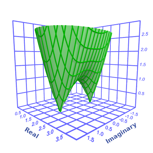
This shows the same information but in 3 dimensions. The bottom plane of the graph is the complex input domain, and the vertical axis represents the modulus of the result. We can see that the roots (where the function touches the zero plane) are still at the same locations.

Both plots are useful. The 3d graph perhaps gives a more intuitive representation, but the color-mapped plot makes it clearer where the roots are located.

Real roots in the complex domain

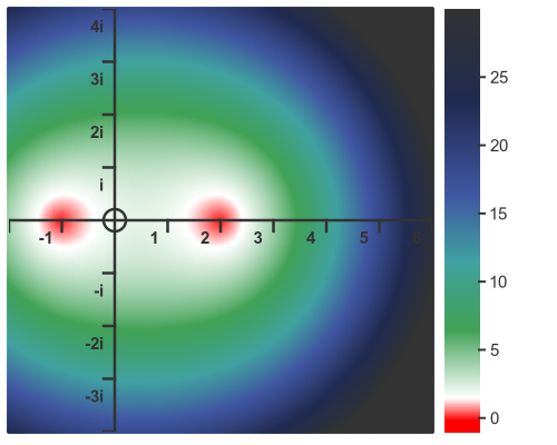
If we look back at our original quadratic equation with real roots:

We can also apply that function to the complex domain. In this case, the roots are both real, with values 2 and -1:

Here is the 3D plot:

Fundamental theorem of algebra

The fundamental theorem of algebra states that every non-constant single-variable polynomial with complex coefficients has at least one complex root.

It is important to remember that a real number is a type of complex number. So considering this polynomial from earlier:

This meets the definition of a polynomial with complex coefficients because 1, -1 and -2 are complex numbers (they just happen to have an imaginary component of zero). Also, the roots of this equation, 2 and -1, can be regarded as complex-valued roots.

Probably the most important takeaway is that if a polynomial has no real roots, it must have at least one non-real root (as in the example we saw earlier). And that this is true even if the polynomial has non-real coefficients (as we will see shortly).

Higher order polynomials

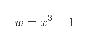
Now let's look at a higher-order polynomial, a simple cubic formula:

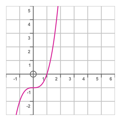
In the real domain this formula has 1 root:

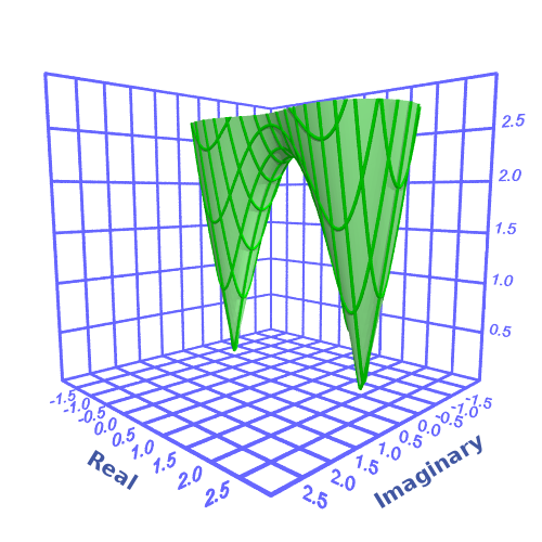
However, if we plot this function in the complex domain, we see there are 3 roots:

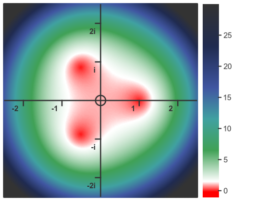
This is no surprise. The solution is the cube root of 1, and the nth root of a number has n complex values.

Non-real coefficients

So far we have only used real coefficients. What happens if we choose non-real values, like this:

Here is the result:

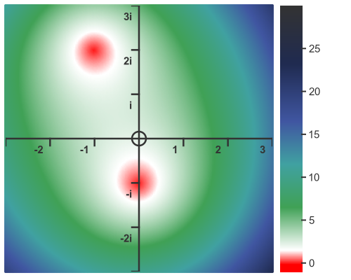
When we change the coefficients in a real-valued quadratic, the curve retains its basic shape, it just gets shifted along the x and y axes. In the complex case, the same thing happens.

One interesting thing is that, with real coefficients, any non-real roots appear in conjugate pairs. That happens, essentially, because all the coefficients are on the real axis, so the initial conditions are symmetrical about the real axis. This means that the final curve (and therefore its roots) is also symmetrical about the real axis.

When we introduce complex coefficients that symmetry is broken. It is then quite common to see complex roots that don't form conjugate pairs.

Plotting the complex value of the curve

So far we have only plotted the modulus of the curve, which doesn't tell the whole story. Every complex number input to a complex polynomial creates a complex number result.

This means the input domain is 2-dimensional, and the output range is also 2-dimensional. We need a 4-dimensional graph! There are various ways to get around this. One is to convert the output values to a single dimension, the modulus, as we have done so far. Another is to create 2 graphs, one showing the real part of the result, and the other showing the imaginary part.

Here is what this looks like for our original quadrilateral with 2 real roots. The real plot is on the left, the imaginary on the right:

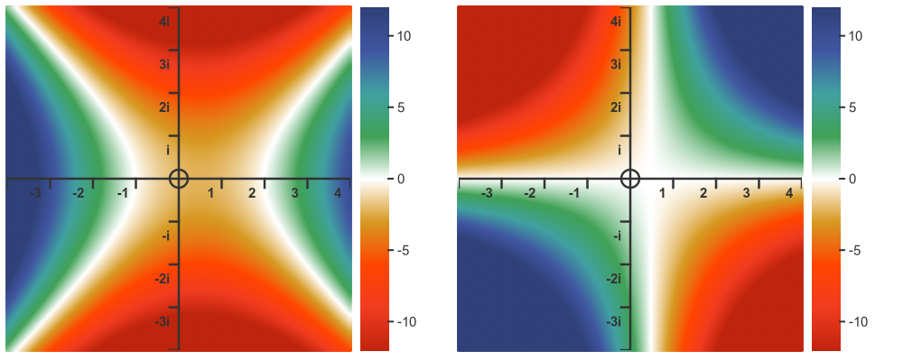
In both of these graphs, the white areas correspond to values that are close to 0. The roots are located where both the real and imaginary parts are both 0. As we know from before the roots are on the real line at -1 and 2, and as expected those points are white on both graphs.

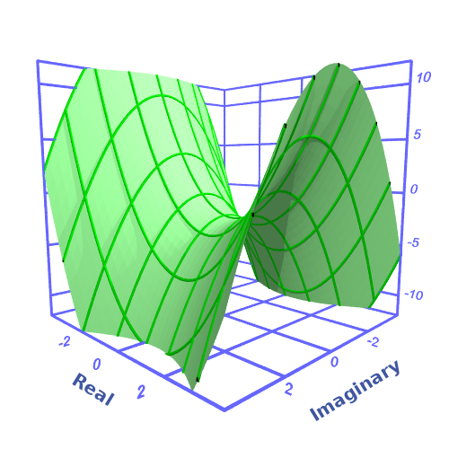
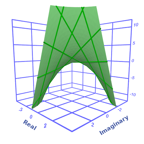
Here is the real part as a 3D plot:

And here is the imaginary part as a 3D plot:

Summary

In this article we have looked at functions in the complex domain, using polynomials as a simple example. We have also seen various ways to visualise complex functions, using colormaps and 3D plots of either the modulus or separate real and imaginary parts.

There is no single best way to visualise complex functions and often a combination of diagrams is useful.

See also

• Imaginary and complex numbers
• Complex number arithmetic
• Argand diagrams
• Why does complex number multiplication cause rotation?
• Modulus-argument form of complex numbers
• i to the power i
• Euler's formula - proof
• Complex powers and roots of complex numbers
• Semiprocal numbers - z to the power i
• Complex number trigonometry functions