What is integration

Integration is a method that can be used to calculate lengths, areas, and volumes defined by mathematical functions. It also has many applications in pure mathematics, physics, statistics, and many other fields. According to the Fundamental theorem of calculus integration and differentiation are (loosely speaking) inverse processes.

This article is an overview of integration. We will look at some of the key concepts but as this is just an overview we will not prove them or explain them in great detail.

Integration as area under the curve

A simple definition of the integral of a function is that it is the area under the curve of that function. Here, on the left, is a simple function, y = 1. The graph on the right shows the area under the curve at every point x:

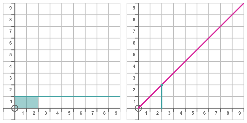
The shaded area in the left-hand graph shows that the area under the curve between 0 and 2 is a rectangle. The rectangle has width 2 and height 1 so its area is 2. The point marked on the right-hand graph shows the value of the integral at that point, which is indeed 2.

In general, the area under the curve between 0 and x is an x by 1 rectangle, so its area is x. The graph on the right, of course, is y = x.

In this next example, the curve on the left is y = 2x:

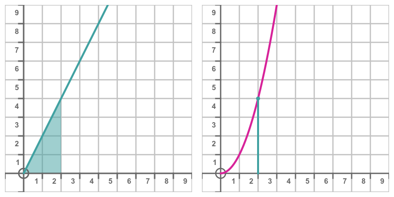
The shaded area under the curve on the left is a right-angled triangle with width 2 and height 4, so its area (half base times height) is 4. The point marked on the right-hand graph shows the value of the integral at that point, which again matches the value 4.

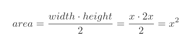
How can we find the formula of the curve on the right? In general at the point x, the width of the triangular area will of course be x, and the height will be 2x (from the formula of the line). So the area will be:

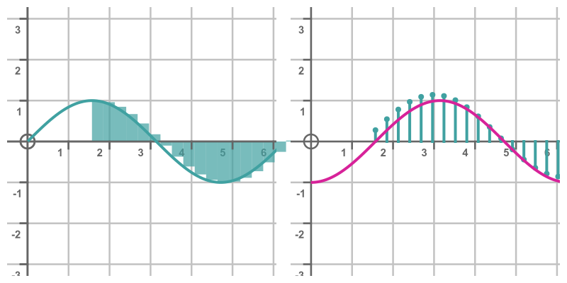
In these simple examples, it was easy to calculate the area using simple geometry. Most cases aren't quite so simple. For example, what is the area under the curve y = sin(x)? It isn't obvious how to calculate this, so one approach might be to approximate the area using rectangles:

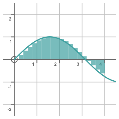
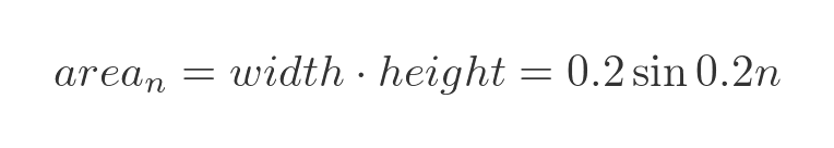
This shows the sine curve, and also a set of small rectangles that approximate the area under the curve. The rectangles in this case have a width of 0.2 - we could choose any value, the smaller the width the more accurate the approximation, but that also requires the sine function to be calculated more often. If we number the rectangles starting from 0, then the nth rectangle starts at x = 0.2 n and has a height sin(x) so its area is:

In the graph below, the cyan stalk plot shows the cumulative total of the areas under the sine curve:

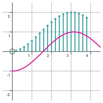
This shape is quite similar to the original sine curve, but shifted in position. In fact, it is related to the function -cos(x), shown in magenta. We will see why they are related, and why they are offset in the y direction, later.

Notation

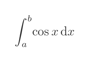
We use the following notation for integration:

where f(x) is some function of x. In the example above we integrated the sine of x:

Fundamental theorem of calculus

The fundamental theorem of calculus tells us that integration and differentiation are inverse operations. In other words, if f(x) is the derivative of g(x), then it follows that g(x) is the integral of f(x).

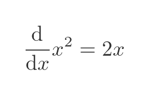
Let's look at one of the previous examples, the case where f(x) = 2x. We want to find g(x) such that the derivative of g(x) is equal to 2x. What function do we have to differentiate to get the result 2x? It is easy to guess:

So the theorem tells us the integral of 2x:

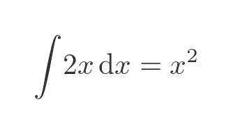
This, of course, matches the result we obtained by calculating the area of the triangle created by the original graph.

We also looked at the integral of sin(x). We could only estimate this geometrically, by drawing rectangles. But we can find an exact result. What function do we need to differentiate to get sin(x)? If you look through any list of derivatives of standard functions you will find useful formula for differentiating cos(x):

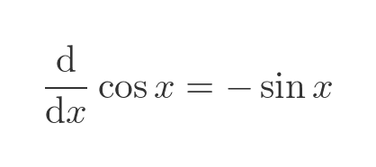
We want sin(x) rather than -sin(x), so we need to negate both sides:

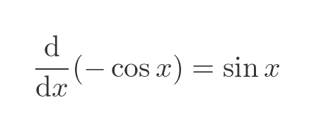
So the integral of the sine function is:

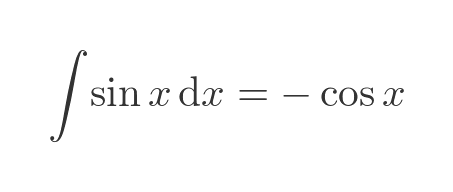
Notice that we almost got this result using the rectangle method. We obtained a curve that looked very much like -cos(x), just offset by 1 in the y direction. We will see the explanation for this discrepancy later.

Standard integrals

As we saw earlier, integrating any particular function f is easiest if we can identify the function g such that differentiating g gives f. We then know that g is the integral of f. Here we will look at a few examples.

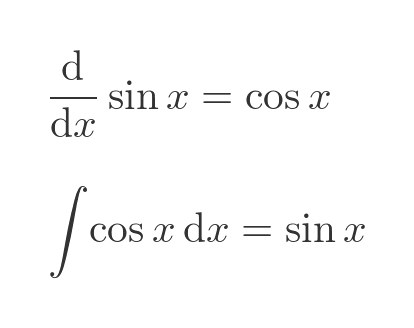
We already know that the integral of sin(x) is -cos(x), and in the same way we can show that the integral of cos(x) is sin(x):

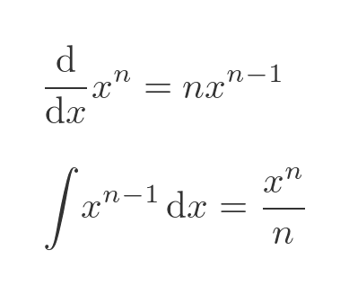
We also know that the integral of 2x is x squared (in other words the integral of x is x squared over 2). We can generalise this to cover other powers:

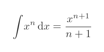
We can write this result in a slightly more useful form by substituting n + 1 for n throughout:

Solving other integration problems

With differentiation, the standard formulas can be derived from first principles. This is how we know the derivatives of polynomials, trig functions, logarithms, exponentials, and so on. These formulas can be combined with other techniques such as the product rule and the chain rule.

Integration works slightly differently. Many of the known standard integrals are derived by inverting a related standard derivative. This is a two-edged sword. On the one hand, it means that every standard derivative result provides a standard integral for free. But on the other hand, to solve a new problem we need to search for a solution rather than being able to directly derive one.

There are also additional techniques that can be applied to standard integrals, which we will touch on later in this article.

The constant of integration

We previously derived the integral of 2x from the following derivative:

But of course, this equation is also valid:

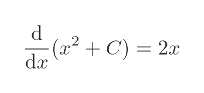
We have added an arbitrary constant, C. When we differentiate, the constant term disappears so the slope is the same. This is a more general equation. The original equation is just a special case of C = 0.

Here are graphs of x squared with different C values. We can see that every graph has the same slope, as shown by the black tangent line on each curve:

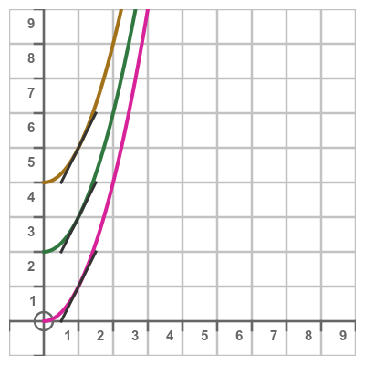
What value of C should we use? Well, they are all equally valid, but the effect of C depends on whether we are using an indefinite or definite integral, as we will see next.

Indefinite integrals

So far, we have specified the integral as a function of x. We have seen that the value represents the area under the curve of the original function, but we have been a bit vague about exactly what that means.

For example, earlier we estimated the area under the sine curve, like this:

We are measuring the area under the curve up to x = 4, but we haven't specified where the area starts. We have just arbitrarily decided to start from 0, but why start there? Why not start at minus infinity? Or 1.5?

This is called an indefinite integral. The integral tells us how the area under the curve changes as x changes, but it can't tell us the absolute area under the curve because we haven't specified where we should start measuring from.

To give an example, suppose we have a car that is travelling along the road between town A and town B which are 30 miles apart, but we haven't been told its exact location. If it travels for 10 minutes at 60 mph how far will it be from town B? Of course, we don't know. We can say that the car is 10 miles closer than it was 10 minutes ago, but we can't say where the car is because we don't know where it started.

If the car was initially at a distance C from town A, it will now be a distance C + 10. But we have no idea what C is. If we were told the value of C (for instance, if the car was initially 5 miles from A) we would then know where the car would be after 10 minutes.

Recall the previous approximate solution to the integral of sin(x), the curve had the shape of -cos(x), but displaced by 1 in the y direction:

We now know that the exact solution to the integral is -cos(x) + C. When we arbitrarily chose to start measuring the area from x = 0 we fixed the value of C at 1. If we had chosen to start from a different point, C would take a different value. If we started measuring the area at π/2, then C would be 0 and the approximate integral would look similar to -cos(x):

Definite integrals

A definite integral has a defined start and end value. It is written like this:

This represents the area under the curve in the range from x = a to x = b. The graph on the left shows this area for the range of 0.5 to 2:

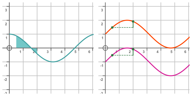
The area is calculated by evaluating the integral at x = 2 and x = 0.5 and calculating the difference. The graph on the right shows the integral function for 2 different values of C. The area is equal to the difference in the y value of the curve between 0.5 and 2, indicated by the solid vertical green line.

Notice, of course, that this distance is the same on both curves, even though they have different C values. This is as you would expect since both curves have the same shape, they are just shifted in the y direction.

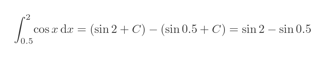
If we evaluate the integral we can see that the C value cancels out when evaluating the integral:

Integration tricks

Various tricks can be used to find integrals of more complex formulas. The first is integration by parts. This is essentially the product rule of differentiation, applied to integration. Sometimes if a function cannot be integrated directly, but can be expressed as a product of two other functions, it allows a solution to be found.

Alternatively, the method of substitution can also be used in some cases. This is the chain rule of differentiation, applied to integration.

Other types of integral

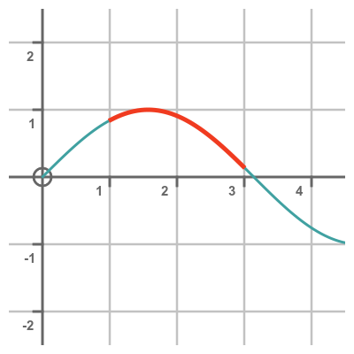
A line integral is used to find the length of the curve rather than the area under the curve. In this case, the line integral would tell us the length of the red curve, which follows the line of the sine curve between 1 and 3:

A surface of revolution is formed by rotating a curve about an axis, often the x-axis. For instance, here is the curve of the square root of x

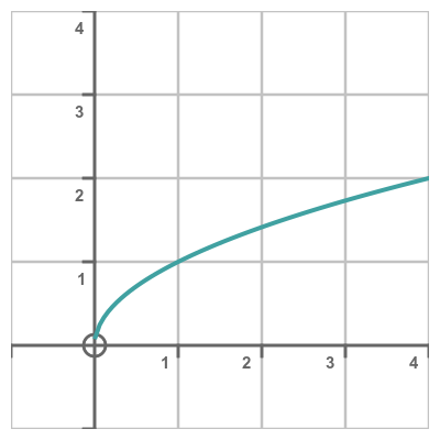
If we rotate this curve about the x-axis we get this 3D shape:

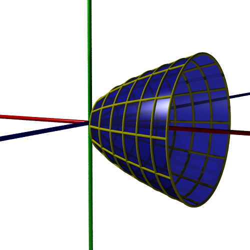
We can use integration to find the surface area of this shape.

A volume of revolution is the volume contained within a surface of revolution. Again, we can use integration to calculate this.

See also

• Integration by substitution
• Mean value theorem for integrals
• Gabriel's horn