Mean value theorem for integrals

The mean value theorem for integrals relates the area under a curve (the definite integral) to the mean value of that curve over the same interval. It is quite a simple theorem, in fact almost obvious, but other important theorems rely on it.

We will start with a graphical illustration before moving on to a precise statement and proof of the theorem.

What is the mean value theorem?

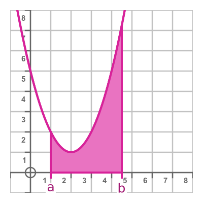
This graph shows the area under the curve f(x) between x-values a and b (ie a definite integral):

Now let's draw a rectangle that has the same width, a - b, as the definite integral. The rectangle has a height v:

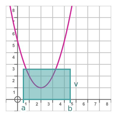
We will choose a value of v such that the area of the rectangle is equal to the area under the curve.

The area under the curve divided by the width of the curve, of course, gives the mean value of the function, so we can conclude that v is the mean value of f(x) over the interval [a, b].

We also know that the top edge of the rectangle must intersect the curve at least once within the interval [a, b], otherwie it would be impossible for the rectangle to have the same area as the integral. We can show this by these two counterexamples:

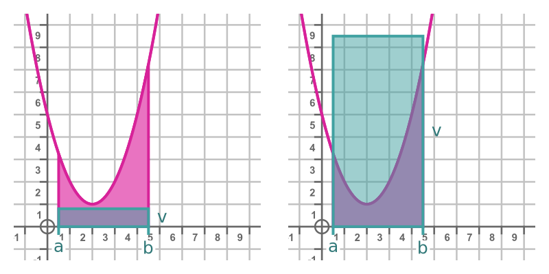
On the left, the rectangle doesn't intersect the curve because its height is too small. The rectangle is completely contained within the area under the curve, so the two areas cannot be equal.

On the right, the rectangle doesn't intersect the curve because its height is too large. The rectangle completely contains the area under the curve, so again the two areas cannot be equal.

So the top of the rectangle must intersect the curve, and in our example that happens in two different places. We can choose one (it doesn't matter which) and call the x-value at that point c.

Of course, we don't know the value of c at this stage. But, since the point of intersection is on the curve, we know that its y-value is f(c) therefore the height of the rectangle is also f(c):

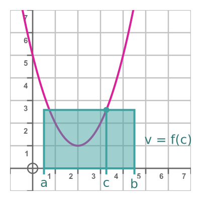
The final result is this. There exists a value c, in the interval [a, b] such that mean value of f(x) over that interval is f(c).

Statement of the mean value theorem

Bringing together what we know so far, we can state the mean value theorem for integrals more precisely.

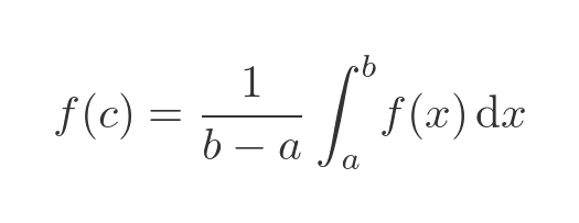
For a function f(x) that is continuous over an interval [a, b], there will be at least one point c in [a, b] such that:

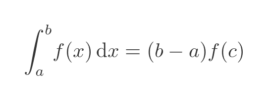
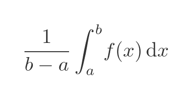
This can also be written as:

The right-hand side represents the mean value of the function.

Supporting theorems required for the proof

The proof of the theorem follows similar lines to the graphical illustration we saw earlier. But the proof relies on three other theorems. They are stated here without proof, but the descriptions provide some justification for them.

All three theorems apply to a function f(x) is continuous over an interval [a, b].

The first is the extreme value theorem. For f(x) there must be a point in [a, b] where f has an absolute minimum value and a point in [a, b] where f has an absolute minimum value. We will call minimum value m and a maximum value M. Here is an example:

It is quite easy to see why this is true. Since f(x) has a continuous set of values over [a, b], there must be a largest and smallest value. Note that this doesn't rule out those values being the same. For example, if f(x) is 1, then the maximum and minimum values are both 1.

The next is the comparison theorem. We know that f(x) is between the min and max values for all x in [a, b]:

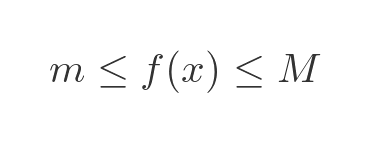
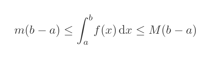
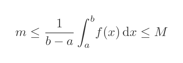
The comparison theorem states that:

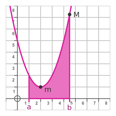
This graph illustrates the theorem. It is quite similar to the graph we used earlier, and demonstrates a similar principle:

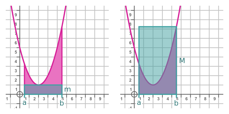
The first term in the equation represents the small rectangle (size m by (b - a)) that just touches the minimum value of the curve. The third term in the equation represents the large rectangle (size M by (b - a)) that just includes the maximum value of the curve. The integral is the area under the curve. As before, the graph shows that this area can't be smaller than the minimum rectangle and can't be larger than the maximum rectangle.

Finally, we will use the intermediate value theorem. This states that, for any value u that is between f(a) and f(b), there will be a value c such that f(c) equals u. It is illustrated here:

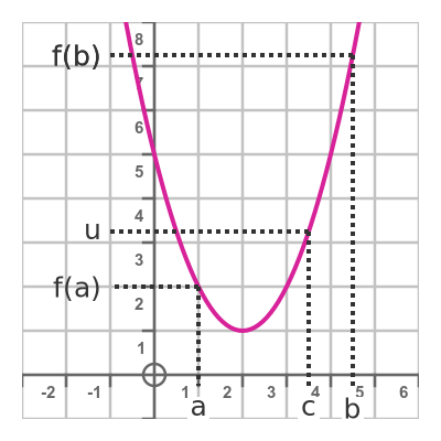
Since f is continuous, it is clear from the graph that wherever we place u (anywhere between f(a) and f(b)) it will map onto some input value c.

Proof of the mean value theorem

We have previously stated that the mean value theorem applies to a function f(x) that is continuous over an interval [a, b], so the theorems above can be applied.

Applying the extreme values theorem tells us that f will have minimum and maximum values, which we will call m and M. This means that:

Using the comparison theorem gives:

Since (b - a) is positive, we can divide through:

Taking the central term:

Since this term has been shown to be between m and M, we can apply the intermediate value theorem, which says that there is some value c such that:

This proves the theorem.

See also

• What is integration
• Integration by substitution
• Gabriel's horn