Permutation matrices and graphs

An adjacency matrix is a way of representing a network or graph as a mathematical matrix.

One of the advantages of representing a graph that way is that computers can process matrices very easily. In this article, we will look at permutation matrices, and see how they can be applied to adjacency matrices.

Identity matrices

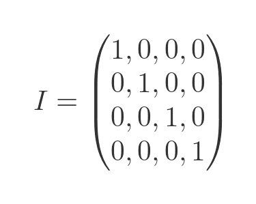
An identity matrix I is a square matrix where all the elements are 0 except for the leading diagonal, where every element is 1. Here is a 4 by 4 identity matrix:

If we multiply another 4 by 4 matrix, A, by the identity matrix I, the result will be A (that is true whether I is placed before or after A):

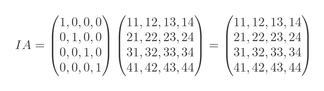
Our matrix has specially chosen values. Each element is a 2-digit number where the first digit is equal to the matrix row, and the second element is equal to the matrix column. So row 1, column 1 has value 11. Row 2, column 3 has value 23, and so on. This means that, when we start moving elements around, we can easily see where they came from.

Before we move on from the identity matrix, it will be useful to look at how it works in slightly more detail. We will replace each diagonal 1 with a variable i1 to i4. These variables will still have a value of 1, but naming them allows us to see which value affects which elements of the result. If we multiply the matrices using the i values we get this:

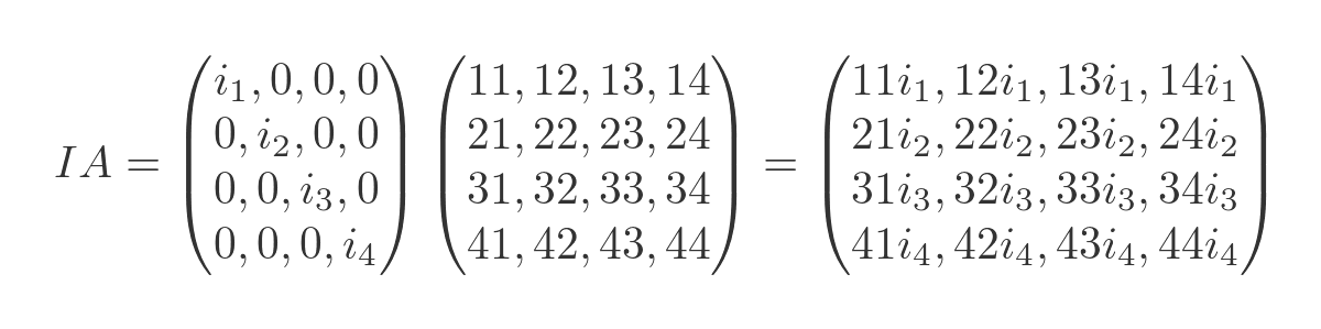
This tells us that the 1 in the first column of the identity matrix is responsible for placing the first row of the source matrix in the first row of the result matrix. The 1 in the second column of the identity matrix is responsible for placing the second row of the source matrix in the second row of the result matrix. And so on.

Permutation matrices - row permutation

A permutation matrix is a matrix where every element is 0, except that there is a 1 in every column and a 1 in every row. The unit matrix is a special case of the permutation matrix, where every 1 is on the main diagonal. Here is a different permutation matrix, P:

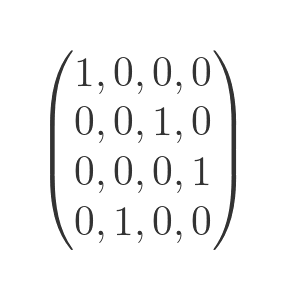
In this matrix, every row has exactly one element with value one, and every row has exactly one element with value one, but the ones are not all on the diagonal.

What happens when we multiply P by A? We get this:

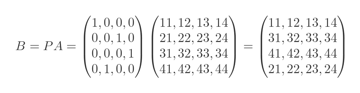
You will notice that the rows of the output matrix are a permutation of the rows of A. We can see the original row from the first digit of each element. This is controlled by the matrix P.

The first row of P has a 1 in column 1, so the first row of A is copied to the first row of B. This is just the same as the identity matrix.

The second row of P has a 1 in column 3. This is different to the identity matrix. This copies the third row of A to the second row of B.

The third row of P has a 1 in column 4, so the fourth row of A is copied to the third row of B. Finally, The fourth row of P has a 1 in column 2, so the second row of A is copied to the fourth row of B.

By adjusting the permutation matrix, we can rearrange the rows of A in any way we wish.

Column permutation

If we reverse the order of the matrices, so that we multiply A by some permutation matrix Q, then the effect will be to reorder the columns rather than the rows. And if Q is equal to the transpose of P, the columns end up in the same order as the rows in the previous example. So:

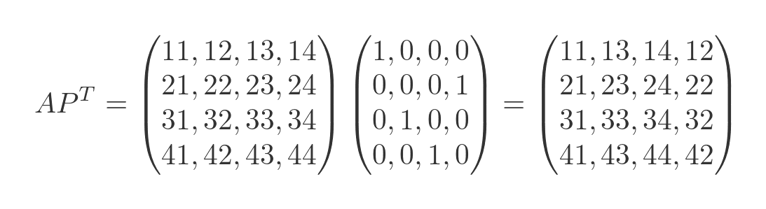
This time we can see that the columns are reordered by looking at the second digit of each element. We won't go into the details, it works in much the same way as row permutation.

Row and column permutations

For analysing graphs, it is often useful to rearrange the rows and columns in the same way. We will see why in the next section.

Based on the previous results, permuting rows and columns is quite simple. We first multiply A by P, then we multiply the result by the transpose of P:

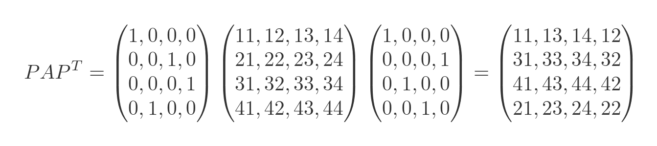
This time, the matrix has been rearranged in both directions. If we choose any column, the first digits of the elements are in the order 1, 3, 4, 2. If we choose any row, the second digits of the elements are in the same order.

Isomorphic graphs

How is this relevant to graphs? We will look at a couple of examples, starting with isomorphic graphs. Two graphs are said to be isomorphic if they are equivalent graphs that differ only because the vertices are named differently, and/or they are laid out differently.

Here is a simple graph, together with its adjacency matrix:

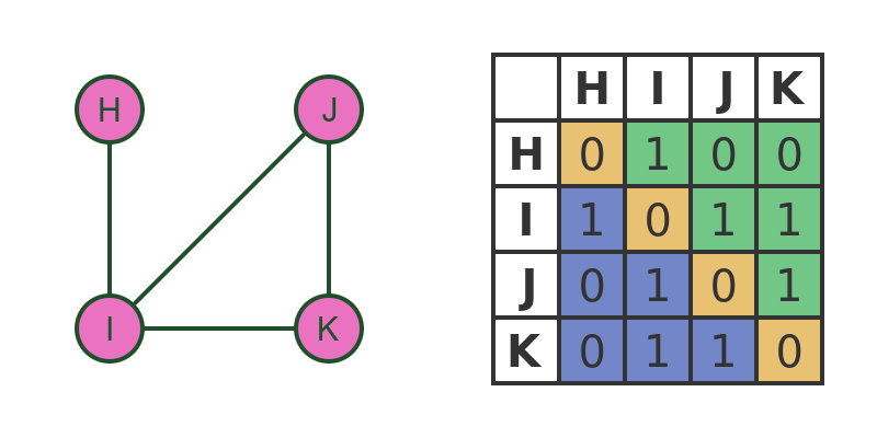
Here is a second graph. It is an isomorph of the original graph, although that might not be immediately obvious from inspection:

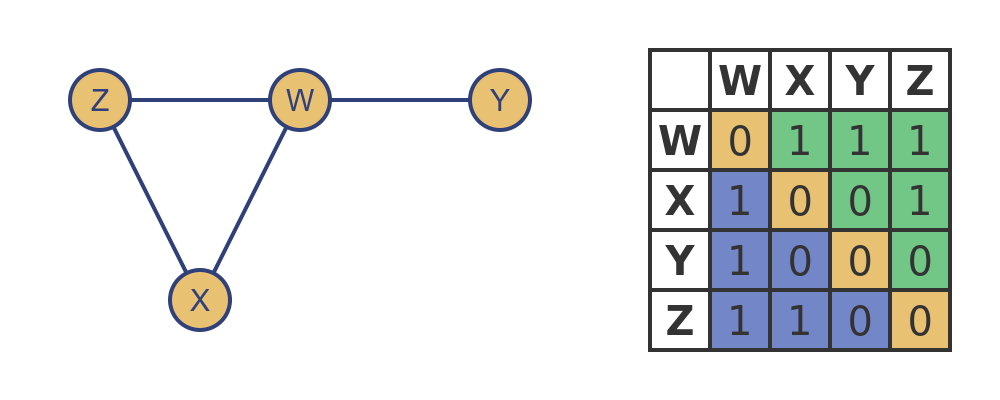
The vertices H, I, J and K in the second graph are directly equivalent to the nodes Y, W, X and Z in the first graph. For a simple graph, we can see that comparing the nodes:

• I is connected to all three other nodes. So is W.
• H is only connected to I. Similarly, Y is only connected to W.
• J and K are both connected to I and each other. X and Z are both connected to W and each other. So J and K are equivalent to X and Z, but notice that in this case, it doesn't matter which way we pair them up. We will match J with X, and K with Z, but it would be just as valid to do it the other way round.

If we now take the adjacency matrix for the second case but rearrange the rows and columns to correspond with the original graph, we get the same adjacency matrix as the original graph:

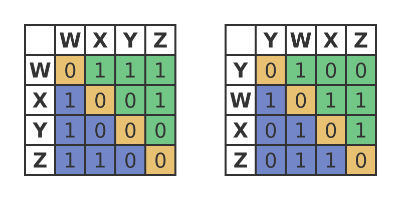
But how do we prove that? Well, the easiest way is to permute one of the adjacency matrices so that the equivalent nodes are in the same order. Since permuting rows and columns doesn't alter the content (the same vertices are still connected together), then if the matrices can be made identical by permuting the rows and columns, it proves that they are isomorphic.

As we saw before, we can do this with a permutation matrix:

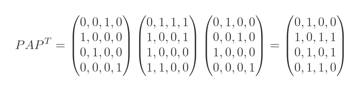
This time the first row of P has a 1 in the third column, so the third row/column (Y) is copied to the first place. The second row of P has a 1 in the first column, so the first row/column (W) is copied to the second place. And so on.

Notice that this technique can be used to easily prove that two matrices are isomorphic if we already know which rows and columns to swap. It won't directly tell us which row and columns to swap, we will need to find that out separately. One way to do that is to perform an exhaustive search, trying every possible permutation matrix and checking for a match. But remember that the number of permutations increases as n factorial.

This creates a similar issue to the brute force solution of the travelling salesman problem. Factorials increase in size very quickly, so for example a graph of 10 vertices can be solved very quickly on a normal PC, a graph of 20 vertices a lot more computing time and power, and a graph of 30 vertices would not be feasible on any current computer.

Bipartite graphs

In a bipartite graph, the vertices can be divided into two separate sets. Vertices from one set can only be connected to vertices in the other set. There are no connections between vertices in the same set.

Here is an example:

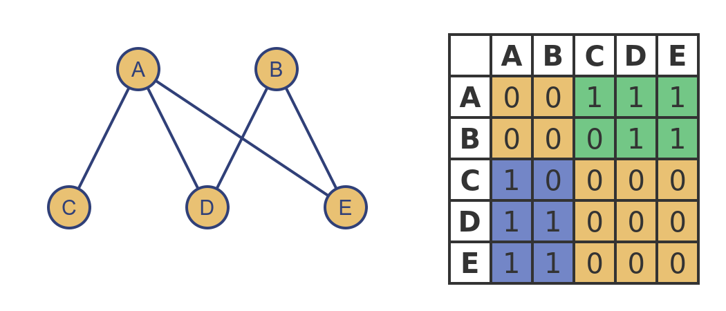
The first set of vertices is {A, B}, the second set is {C, D, E}. Notice that A is not connected to B. Also, there are no connections between C, D, and E. The only connections are between vertices that are in different sets.

This is also clear from the adjacency matrix. The two yellow areas represent the two sets. The square area in the upper left represents connections between A and B, and of course every element is 0. The square area in the lower right represents connections between C, D, and E, and again every element is 0. This is a classic signature of a bipartite graph, the top left and bottom right areas are all zeroes.

But that is only apparent if the vertices are ordered sensibly. Here is an isomorph of the graph above, with the vertices renamed in a different order:

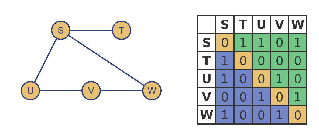
This is still a bipartite graph because it is isomorphic with the original. But it is harder to see because of the ordering. It is more difficult to see the groups in the graph diagram, and we don't see the signature zeros in the matrix.

As before, we can make this far clearer by applying a permutation matrix to reorder the vertices. The matrix isn't shown here, but the transformation is quite simple in this case. We just need to swap the V and T rows and columns in the matrix. For good measure, we have also rearranged the vertex positions in the graph diagram as well:

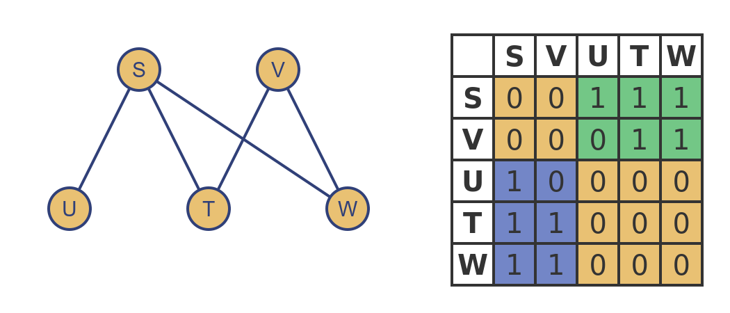
Again, this doesn't tell us which rows and columns to swap to put the graph into its clearest form, but if we know what change we need to make they provide an efficient way of transforming a graph.

See also

• Graphs
• Adjacency matrices
• The seven bridges of Königsberg
• Dijkstra's algorithm
• Travelling salesman problem