Graphs

Graph theory has many uses in mathematics, computer science, and other fields.

What is a graph?

In graph theory, a graph is a collection of vertices connected together by edges, like this:

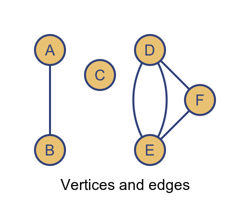
As a concrete example, each vertex might represent a different town, and the edges might represent the major roads connecting the towns.

Vertices are represented by circles. Each vertex usually has a unique name, such as the name of the town. In this article, we will use single letters or digits to identify vertices.

A vertex can be connected to any number of other vertices, or none at all (like vertex C above).

Edges are represented by lines between the vertices. An edge is identified by the vertices it connects to, for example, if the edge represents a road, it might be identified as the road from town A to town B. Edges can sometimes have extra information, such as the length of the road.

Edges usually connect one vertex to another, although it is sometimes possible for an edge to connect a vertex to itself - this is called a loop. An edge can never connect more than two vertices.

Here are some commonly used pseudonyms:

• Graphs are sometimes called networks.
• Vertices are sometimes called nodes or points.
• Edges are sometimes called lines, links, or arcs

Applications of graph theory

Graph theory can be used wherever we need to represent the connections between different things, for example:

• Towns connected by a road or rail network.
• Devices on a computer network.
• The atoms in a complex molecule.

We can perform algorithms on graphs, for example:

• Finding the shortest route between two towns connected by a road network.
• Optimising a set of tasks, where a graph shows dependencies between the tasks.

Graphs can indicate the structure of data, for example:

• The grammar of a statement in a computer programming language.
• A family tree.

There are many other uses.

Types of graphs

There are several different types of graphs. A simple graph is a graph where there is at most one edge between any pair of vertices, like this:

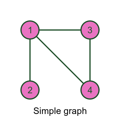
Here, for example, there is one edge between vertex 1 and vertex 2. But there is no edge between vertex 2 and vertex 4.

A multigraph is a graph that permits more than one edge between a pair of vertices, like this:

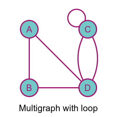
In this case, there are two edges between C and D, which makes the graph a multigraph.

This graph also includes a loop - the vertex C is connected to itself. Not all graphs allow loops. For example, it would make no sense to have loops in a family tree, because you can't be your own parent. If a graph allows loops we call it a multigraph permitting loops (or a simple graph permitting loops).

For the graphs above, the edges have no direction. For example the edge between A and B is exactly the same as the edge between B and A. There is no distinction.

In a directed graph (sometimes called a digraph) edges have a direction, like this:

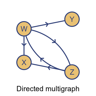
In this graph, every edge has an arrow giving it a direction. So for example the link from W to Y only goes in one direction. It is like a one-way street, you can use it to get from W to Y but not from Y to W.

However, there are two links between W and Z, with arrows in opposite directions, so it is possible to travel in either direction. The fact that there are two edges makes this graph a multigraph.

Another type is a weighted graph. In this type of graph, each edge has a numerical value associated with it, called a weight. The weight can represent any relevant quantity. For example, if the vertices are towns and the edges are roads, it might represent the distance between the towns.

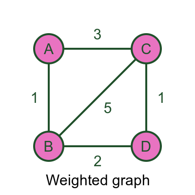
With weighted graphs, we can solve optimisations problems such as finding the shortest route from A to D. This would be ABD, with a distance of 3, which is shorter than ACD with a distance of 4.

We can also combine these different types of graphs. For instance, we can create a weighted, directed multigraph like this:

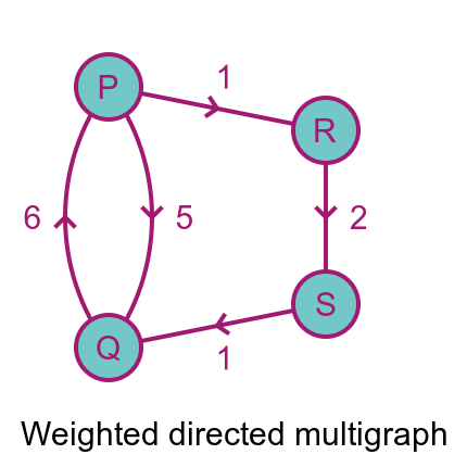
The shortest distance from P to Q is PRSQ with a distance of 4 because going directly from P to Q has a distance of 5.

But, going the other way, the shortest distance from Q to P is 6 going directly from P to Q. It isn't possible to go via S and R because the edges have the wrong direction.

Subgraphs

If we have a graph G, a subgraph of G is any graph where all the vertices and edges are part of G, like this:

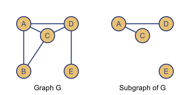
In this case, the vertices (A, C, D, and E) of the right-hand graph are part of graph G. And the edges AC and AD are part of G. So the graph is a subgraph of G.

There are some special subgraphs. The simplest is a path. A path is a sequence of edges, joined end to end, that connect two particular vertices. A path must not pass through the same vertex twice:

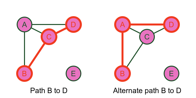
For example, there is a path from B to D via C. This uses the edges BC and CD to connect B and D.

This path is not unique. We could also travel from B to D via A, which is a different path with the same start and end points.

Notice that there is no path from B to E.

A walk is like a path, except you are allowed to visit the same vertex more than once. So for example if you travelled from B to D using BCABCD that would not be a path because it visits B and C more than once. It would be a walk.

Every path is a walk, but not every walk is a path.

A cycle is similar to a path, except that the last edge joins onto the first vertex of the path, like this:

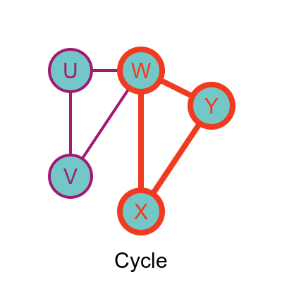
In this case, the vertices WXY form a cycle (sometimes called a circuit). It isn't always possible to form a cycle, depending on the edges of the graph.

Another important subgraph is the spanning tree, but we will defer that until we have looked at trees.

Special graphs

There are several special types of graphs that are very useful.

In a connected graph there is a path between every pair of vertices:

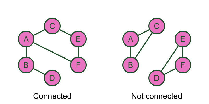
In the connected graph, starting from any vertex, there is a path to any other vertex.

In the not connected case, some of the vertices have no path between them. In the example shown, there is no path between C and E. In fact, the graph is divided into two separated regions, ABC and DEF. There are paths within each region, but no paths between the regions.

Generally, if a graph is not connected, there will be some combination of:

• Separate regions where each region is a connected graph, and/or
• Isolated vertices that have no edges at all.

A complete graph has an edge between every pair of vertices, like this:

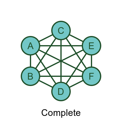
In a complete graph, it is possible to move from any vertex to any other vertex directly, using just one edge.

A tree is a connected graph that contains no cycles:

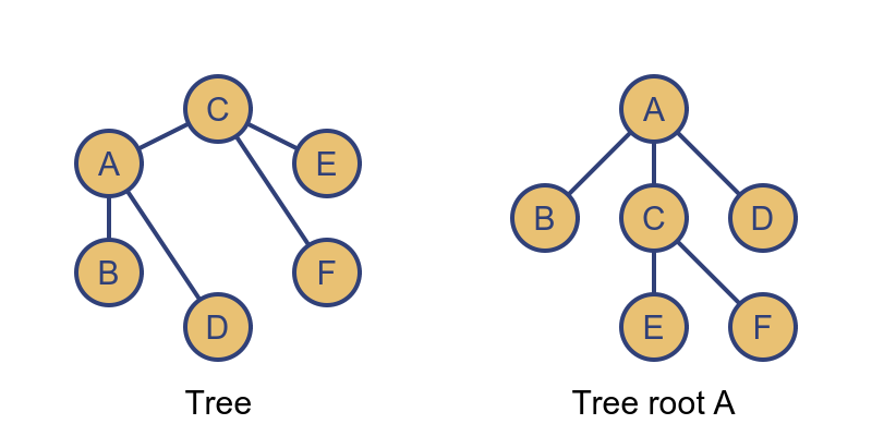
A tree can be rearranged so that one vertex is at the top (A in this case) and the other vertices fan out below it. In fact, a tree can be rearranged so that any vertex is in the top position. Here is the same graph with F at the top:

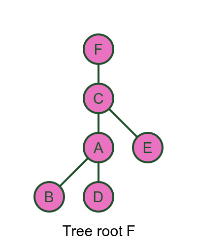
These two trees are isomorphic - they contain the same vertices and edges, just laid out differently. We will meet this term later.

We mentioned spanning trees earlier. If we have a connected graph that might contain cycles, we can create a tree that includes all the vertices but with no cycles:

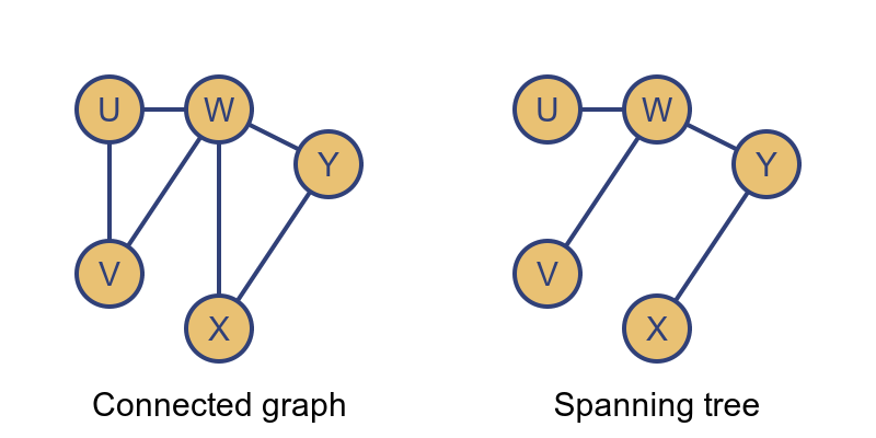
The spanning tree has all the vertices, but we have removed enough edges to ensure that there are no cycles. This leaves a tree that contains every vertex of the original graph. The advantage of the spanning tree is that we can traverse the tree to visit every vertex exactly once, without having to worry about cycles.

A bipartite graph is one where the vertices can be divided into two sets. Here the vertices A, B, and C are on the left, and the vertices X, Y, and Z are on the right:

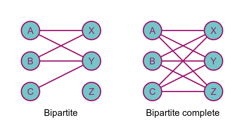
There are edges between the two sets of vertices, but there are no edges within either set of vertices. There are no edges between A, B, and C. There are no edges between X, Y, and Z.

The second graph above shows a bipartite complete graph. In this graph, every vertex on the left has edges that connect to every vertex on the right.

Note that a bipartite complete graph is not the same as a complete graph. A complete graph would have extra edges between the vertices on the left, It would also have extra edges between the vertices on the right.

Finally, we will look at isomorphic graphs. Two graphs are isomorphic if they have exactly equivalent vertices and edges. For example:

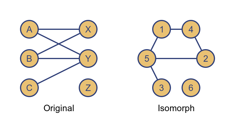
In these two graphs, the vertices are named differently, and the graph is arranged differently, but the two graphs contain the same information. The bipartite layout makes it easier to understand the nature of the graph, so it is arguably better from that point of view.

Properties of vertices

We will return to the graph from the start of the article, to look at properties of vertices.

We say that two vertices are connected if there is a path between them.

So A is connected to D because there is an edge joining them. But also B is connected to C because there is a path BDC between them.

The degree of a vertex is the total number of edge endpoints that connect to it.

So B has a degree of 2 because there is an edge connecting it to A and another edge connecting it to D. D has a degree of 4 because it has an edge connecting it to A, and to B, and then 2 edges connecting it to C.

C is a little more tricky. It has a degree of 4 because it has 2 edges connecting it to D, and also a loop connecting it to itself. A loop counts as 2 edges because both ends of the loop edge connect to C.

The degree of a vertex is sometimes called its order or valency.

We also talk of vertices having odd or even order, based on whether the order is odd or even. All the vertices in the diagram above have an even order because their order is either 2 or 4.

Adjacency matrix

Graphs can also be represented using an adjacency matrix. Here is a simple graph represented as a graph diagram and a matrix:

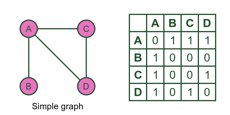
The value of the matrix at (i, j) is 1 if there is an edge between vertices i and j, and 0 if there is not.

So row A, column B is 1 because there is an edge between A and B.

Row B, column C is 0 because there is an edge between B and C.

The adjacency matrix of a simple graph has the property that the value at (i, j) is equal to the value at (j, i). This is because if there is an edge between vertices i and j, there is also an edge between vertices i and j (it is the same edge, of course). For example the edge between A and B is also an edge between B and A.

A matrix that has the property that the value at (i, j) is equal to the value at (j, i) is called a symmetric matrix. Undirected graphs have symmetric adjacency matrices.

For a directed graph, the situation is slightly different:

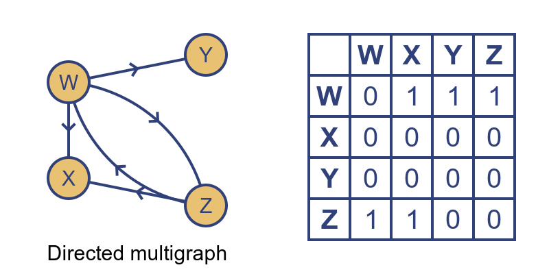
In this case, the matrix is not symmetric. For example, row W column X is 1 because there is an edge from W to X. But row X column W is 0 because there is no edge from X to W. That is because the edge from W to X only exists in one direction.

Weighted adjacency matrix

The concept of adjacency matrix can be extended to include weighted graphs, like this:

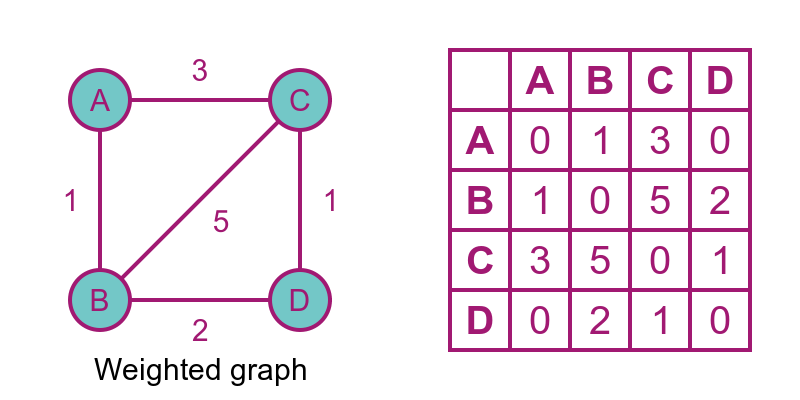
In this case, each element in the matrix species the weight of the edge between the corresponding vertices. For example, row A column C has a value 3, because A and C are linked by an edge of weight 3.

We use the value 0 to indicate that there is no edge between the corresponding vertices.

See also

• Adjacency matrices
• The seven bridges of Königsberg
• Dijkstra's algorithm
• Travelling salesman problem