The erf function

The error function is a special function that is related to the normal distribution (also known as the Gaussian distribution).

The error function is closely related to the cumulative distribution function (CDF) of the normal distribution. As we will see, this function involves an integral that cannot be solved by the usual methods. The error function, written as erf(x), was introduced as a special function that solves the integral.

It also turns out that the error function can also be used to solve other, general integrals that take a similar form.

In this article, we will cover both of these aspects of the function, starting with an overview of the normal distribution.

The normal distribution

The normal distribution is a probability density function (PDF). Here is a graph of the normal distribution, on the left:

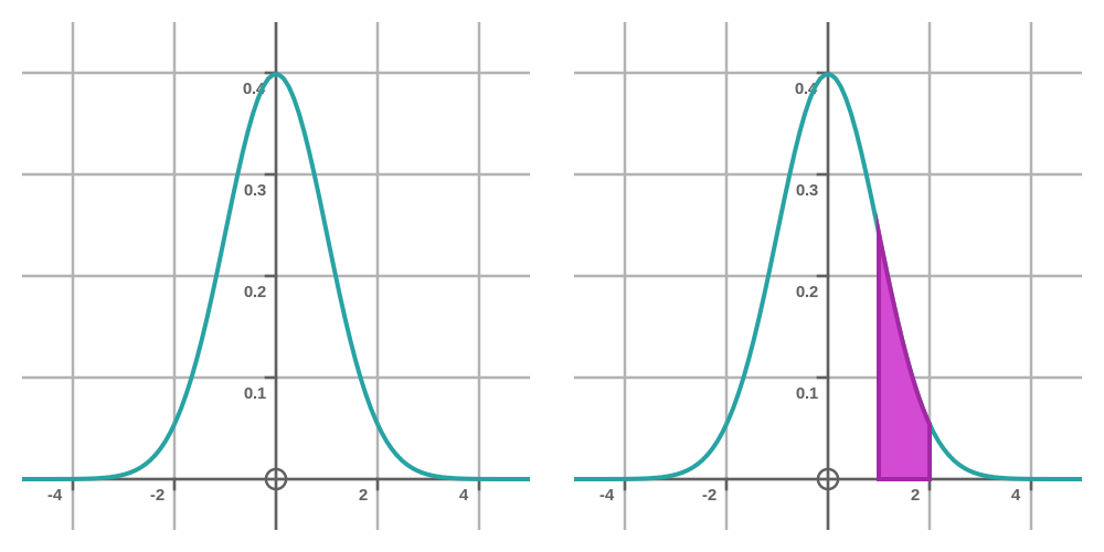
We will use a simple example to understand how to interpret this graph. Let's say the graph relates to a bus service, and the x-axis represents the arrival time of the bus. Zero represents the bus being on time, 2 represents the bus being 2 minutes late, and -2 represents the bus being 2 minutes early, and so on.

A PDF tells us the probability of the bus turning up within a certain range of times. For example, what is the probability that the bus will be between 1 and 2 minutes late? Well, the graph on the right, above, shows this. The probability that the bus will arrive within this time frame is given by the area under the curve, between x = 1 and x = 2, shaded in magenta on the graph.

The magenta area has a width of 1, and its height starts at around 0.25 and falls to around 0.05. Since it is roughly trapezium-shaped, we might estimate its average height to be 0.15. With a width of 1, that means its area will be about 0.15.

So the probability that the bus will be between 1 and 2 minutes late is 0.15, or 15%.

If we assume that the bus is bound to arrive sometime, we can say that the total area under the curve is exactly 1.

The formula for the normal distribution

The graph above has the equation:

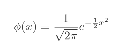
This is the standard normal distribution. The mysterious division the root of 2π is there to ensure that the area under the curve is exactly 1. The formula applies to distributions where the mean is 0 and the standard deviation is 1. See the linked article for more information about the general normal distribution.

This curve is based on the following, simpler function that produces the basic bell shape. We will refer to this as the bell function when we use it again later:

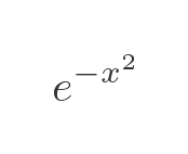
It produces this curve:

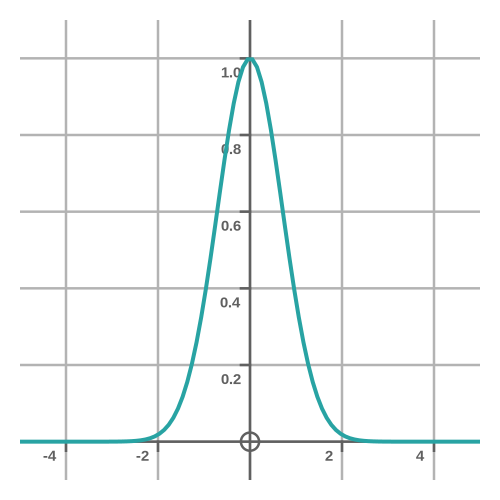
The main difference between the simple bell curve and the normal curve is that the normal curve is divided by a factor of root of 2π, as described earlier. There is also s small difference in the exponent, the normal function has an extra factor of 1/2.

Cumulative distribution functions

As we saw, the probability that the bus is between 1 and 2 minutes late is given by the area under the PDF curve between those points. The cumulative distribution function (CDF) makes this easier.

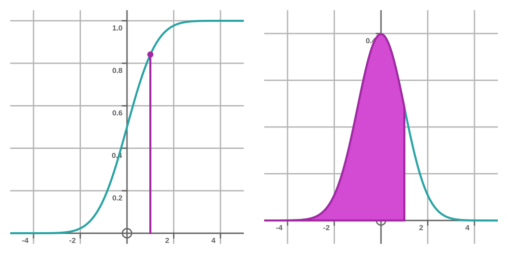
The CDF is a curve that tells the probability that the bus will arrive at or before a certain time. For example, the CDF value of 1 minute is the probability that the bus will not be more than 1 minute late. That is to say, the bus might be 1 minute late, or 30 seconds late, or on time, or 5 minutes early, etc. The value of the CDF at 1 minute is equivalent to the area under the PDF from 1 minute right back to minus infinity:

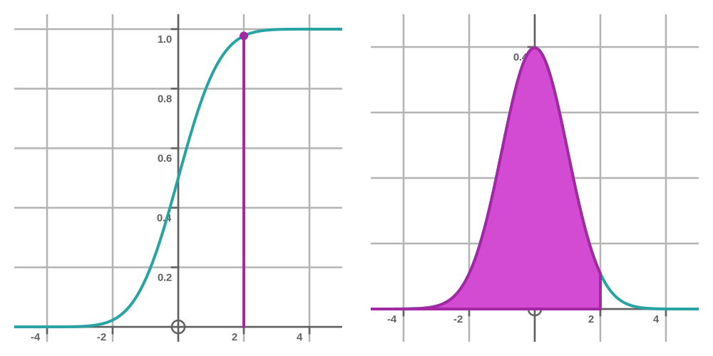
Likewise, the value of the CDF at 2 minutes is equivalent to the area under the PDF from 2 minutes right back to minus infinity, ie the probability that the bus will not be more than 2 minutes late:

What is the probability that the bus will be between 1 and 2 minutes late? In terms of the PDF, it is the area under the second curve, minus the area under the first curve. In terms of the CDF, it is just the difference between the two values at 1 and 2 minutes:

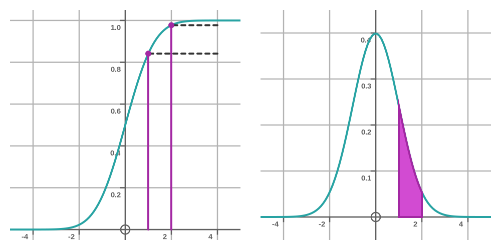
In other words, the probability is the y-distance between the two dashed black lines. Looking at the graph, we can see that the gap is about 0.15, the same as our previous estimate of the area under the PDF.

How do we find the CDF? Well, it is just the area under the PDF curve. We find the area by integrating the PDF function from earlier:

This is great except for one small problem. We can't solve the integral using elementary functions such as sine, log, etc.

The error function, erf

Often, when faced with an integral that cannot be solved in the usual way, we define a special function that solves the integral. Examples of special functions include the gamma function and the Lambert W function. These special functions have been widely studied and are well understood, and we have numerical methods for calculating the value of the function to many decimal places.

Essentially, if we can find a solution to an integral in terms of a special function, then we can consider it fully solved (in the same way that if we can find a solution to an integral in terms of the trig functions, we consider it fully solved).

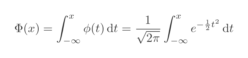
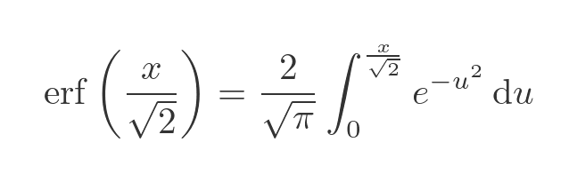
We could solve the previous integral for the CDF, Φ(x), simply by declaring Φ to be a special function. But that wouldn't be ideal, because that function is a bit too specific to the normal distribution. Instead, we use a slightly more general function, called the error function, or erf(x). This is defined as:

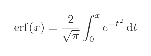
Comparing this with the previous Φ function, there are a couple of simplifications:

• The erf functions uses the definite integral over the range 0 to x, whereas Φ uses the range -∞ to x (an improper integral, which can make things more complicated).
• The Φ function has a factor of 1/2 in the exponent. The erf function is based on the simpler bell function from earlier, which has no extra factor in the exponent.

We have also adjusted the multiplication factor. It is now 2/√π. This is done so that the erf function tends to 1 as x tends to infinity.

Plotting the erf function

Looking at the definition of erf, it might initially appear that it is only defined for x >= 0, because the integral limits are 0 to x. This is plotted on the LHS of the graph below. Notice that when x is 0, the function is 0, because a definite integral from 0 to 0 is 0. As we saw earlier, the curve has a horizontal asymptote at 1 as x gets large:

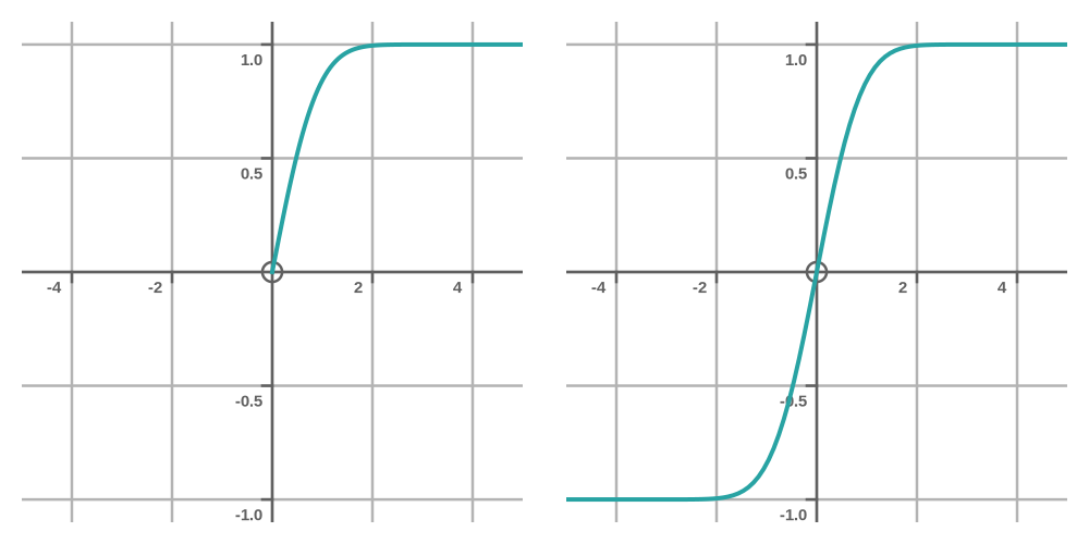
What about x values that are less than 0? Well, the integrand in the erf function is the bell function from earlier, and the bell function is an even function (that is, it is symmetrical over the y-axis). There is a general rule that if we integrate an even function, the result is an odd function. So we can say that:

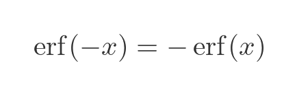
This allows us to complete the graph of erf, shown on the RHS of the graph above.

Expressing the normal function in terms of the error function

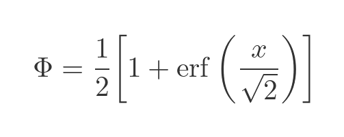
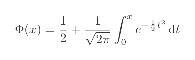
The previous expression for the normal CDF Φ and the error function erf look quite similar, and in fact, we can express Φ in terms of erf like this:

This can be shown fairly easily by a few manipulations of the Φ formula. Taking the formula for Φ from earlier, we first split the integral into two parts, the integral from minus infinity to 0, and the integral from 0 to x:

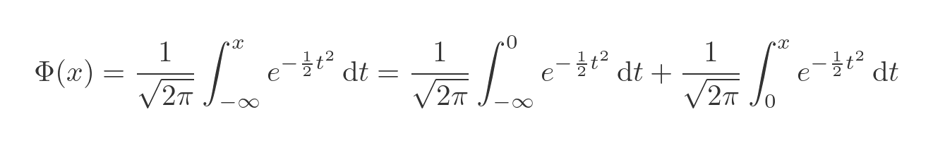
Notice that the first integral, from minus infinity to 0, represents the area under the normal curve for x less than 0. Since the normal curve is symmetrical about 0, and has a total area of 1, that means that the first integral evaluates to exactly 1/2:

What about the second integral? This looks a bit like the erf function, except for the troublesome factor of 1/2 in the exponent. But we can write the exponential term as:

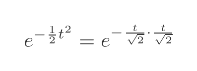
This allows us to perform a simple u-substitution (change of variables) like this:

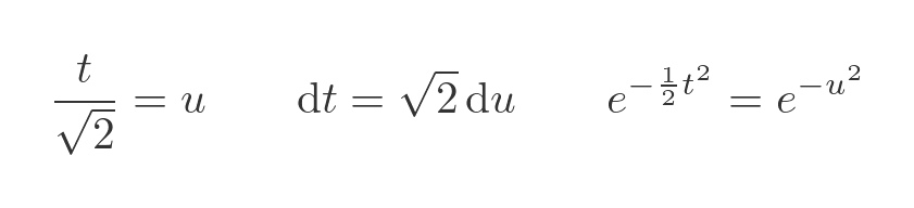
Putting this change back into the integral gives:

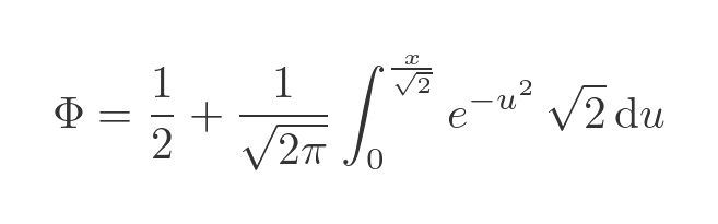
Notice that we have also adjusted the upper range of the integral to x divided by root 2, because of the change of variable. The integral can be simplified to this:

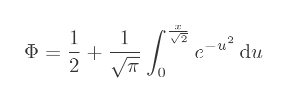
From the definition of the erf function, we know that:

This is the same as the previous integral term, just multiplied by 2. This demonstrates the result:

Calculating the erf function

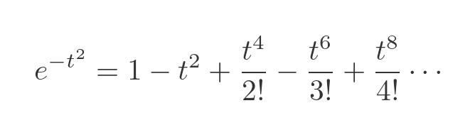
Since the erf function cannot be expressed in terms of the more commonly known elementary functions, we need to find a way to approximate the function numerically. One way to do this is to use a Maclaurin expansion. In particular, the expansion of the exponential function. Referring to the linked article, we can express the exponential function as an infinite polynomial. This is a standard formula:

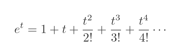
We are interested in the exponential of -t², which can be found by substituting -t² for t in the formula:

The erf function is related to the integral of this exponential, from 0 to x. We can integrate both sides:

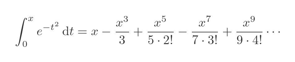
We have made use of the fact that every term has a factor of x, so the integral evaluated at 0 is 0, and has been discarded. Recall that the erf function is equal to this integral multiplied by 2 over root pi. We can also simplify the denominators, giving us:

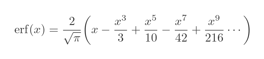
This, in principle, can be used to calculate the erf function for any value of x. But in practice, it can be slow to converge for larger values. Several other methods converge faster over certain ranges of x. Practical implementations, for example in software maths libraries, often use different methods for different ranges of x values.

Solving integrals with the erf function

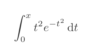
Finally, we will look at how we can use the erf function to solve a tricky integral. Here is the integral:

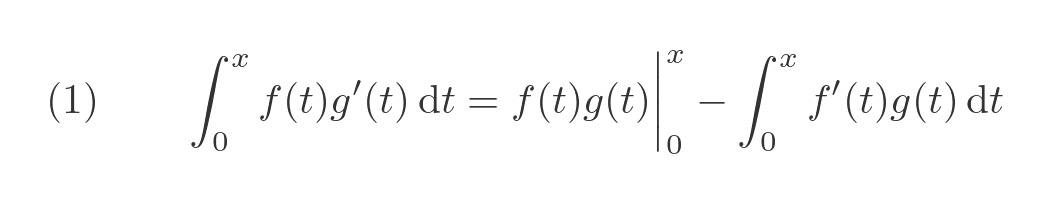
Since this is the product of two terms, we might try integration by parts. The formula for this is:

We need to split our integrand into two parts, f and g'. We might do it like this:

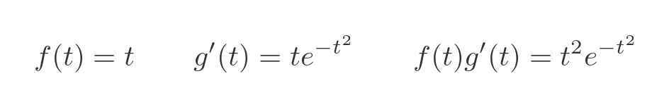
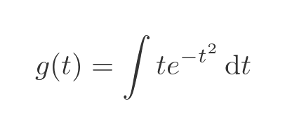
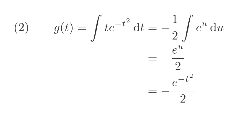
Why split it like this? Well, we will need to differentiate f and integrate g'. If we differentiate f, we get 1, which is nice and simple. And g' looks like a good candidate for integration by substitution. Let's start with that:

We can use the following integration by substitution subsitution to simplify the exponential and get rid of the x term in the integrand:

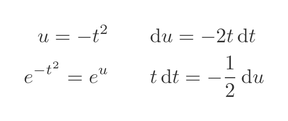
Here is the result:

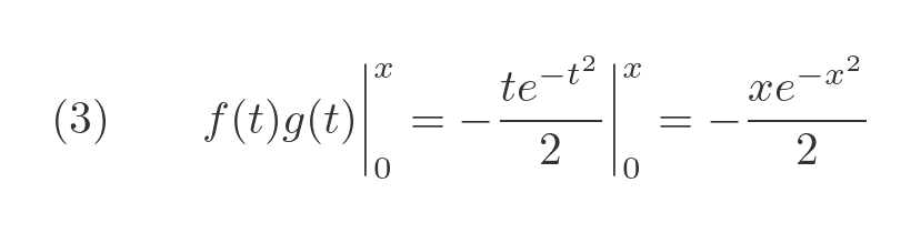
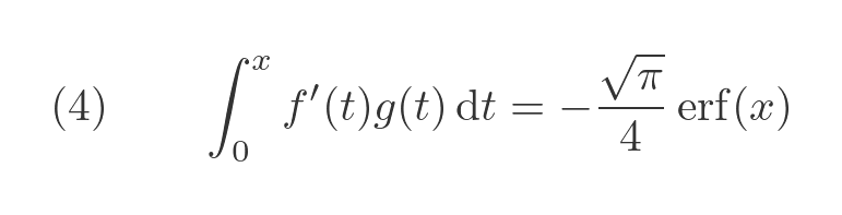
Now we know g we can find both terms in equation (1). The first term is:

The second term is also quite easy to find. Since f' is 1, it is simply the integral of g:

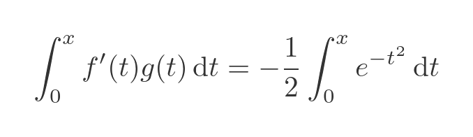
This, of course, looks very much like the erf function. Which is quite fortunate, because there is no other way to find a solution to this integral. Looking at the definition of the erf function, we express the integral above in terms of erf:

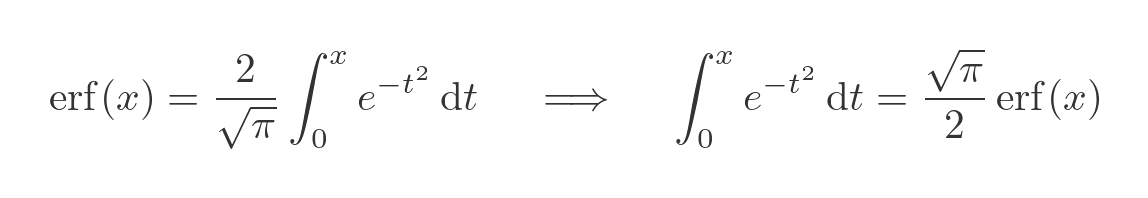
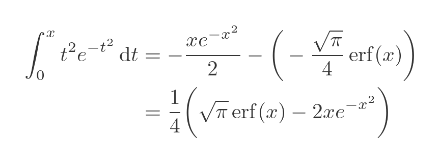
This gives a final expression for the second term:

Combining the results of equations (3) and (4) into the original equation (1), and simplifying, gives the answer:

See also

• The pi function
• The Lambert W function