The pi function

The factorial function n!, is a well-known function that has many applications in mathematics. It is defined for non-negative integers as:

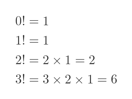
The normal definition of the factorial defines a process for calculating n!. You must multiply together every integer from 1 to n. In the early 18th century, Euler and several other mathematicians attempted to find a function that would return the value of n! when passed any non-negative integer n.

The answer they came up with was the pi function Π(x) (nothing to do with the mathematical constant 3.414..., pi is just the Greek letter, it is capital form Π). This function has been largely consigned to history since Euler invented the gamma function shortly afterwards. But it is still interesting, firstly because it was a crucial step to finding the gamma function, and secondly because it is very clever in its own right.

So the requirement of the pi function is that:

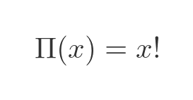
For all non-negative integer values of x.

There is no obvious function that meets this specification, it required a bit of creative thinking.

The pi function

Euler and his collaborators discovered a function that fits the bill. Here is the pi function, which can be used to find the factorial of any non-negative integer value of x:

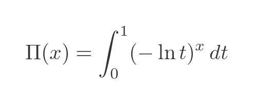
In this section, we will only look at how the pi function works. The proof will be left until the end - it isn't difficult to prove, but a little long-winded, so it is good to get a feel for how it works first.

The first thing to realise is that this is a function of x, not a function of t. The variable t is only used within the definite integral. If we use a different x value, the function being integrated is different. So the result of the integral only depends on x.

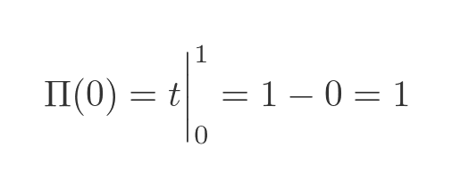
To illustrate this, consider the situation when x = 0. The resulting integral is shown below. Since the log term is raised to the power 0, it simplifies to 1 (anything to the power 0 is 1):

The integral of 1 is simply t. We find the definite integral by evaluating t at 1 and 0, giving the result 1:

Now let's try the same thing with x = 1. Raising anything to the power 1 leaves it unchanged, so we can just discard the power. Notice we have moved the negative sign outside the integral:

We can solve this using integration by parts. The full workings are shown at the later in the article, but the end result is:

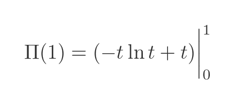
This has a log term, so you might think it is unlikely to give an integer result. But the limits of the integral have been chosen very carefully:

• When t is 0, any term multiplied by t will be 0.
• When t is 1, ln t is 0, so any term multiplied by ln t will be zero.

Combining these conditions, we can see that the term t ln t is 0 when t is either 0 or 1, so the term can be discarded when we evaluate it between 0 and 1. So the function simplifies to:

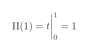
Now let's do it again for x = 2:

Again we will use integration by parts, together with the chain rule (this is also shown in detail at the end of the article):

There are two important points to notice here:

• The factor of 2 before the integral term arises because the log function is squared (it appears when we apply the chain rule).
• The integral part of the expression is identical to the negative of Π(1). So -2 times the integral is equal to 2Π(1).

Once again, any term that involves both t and ln t disappears when evaluated at 0 and 1, giving:

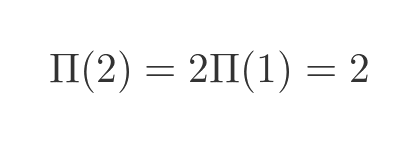
Doing the same again for x = 3, we have:

The integral works in a similar way. The factor of 3 comes from applying the chain rule to the log cubed term:

We eliminate the terms in t and ln t, giving:

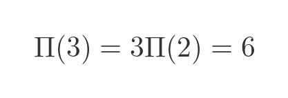
At this point, a clear pattern is emerging. Each time x increases by 1, the result is x times Π(x - 1), which of course gives the factorial.

Isn't this a bit of a cheat?

This might seem like a bit of a cheat. Sure, we have a nice function that can tell us x!. But to use it, we have to evaluate a string of nested integrals. And the end result of that is to multiply x times x - 1 times x - 2 ...

So it is just a more complicated way of finding a factorial by multiplication.

There are a few ways to answer this. First, the challenge was to find a function that evaluates factorials. Nobody said it had to be a more efficient way of calculating factorials. There might not even be a more efficient way.

Second, we now have a simple formula for calculating factorials that we didn't have before, which is pretty amazing. And regardless of the practical difficulties in calculating it, the fact remains that the function still holds:

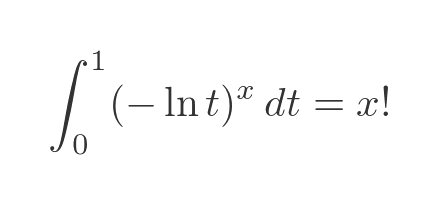
This gives us a whole new way to calculate a factorial. We can use a numerical method, such as Simpson's rule, to approximate the integral. And it works (why wouldn't it?). Which again is pretty amazing. Although, in practical terms, this method isn't very useful as it converges very slowly.

However, the most important implication of this method is that it leads directly to the gamma function, which is inarguably useful in many applications.

The value of t ln t

As an aside, we previously used the fact that t ln t is 0 when t is 0.

You might have spotted a potential problem with this. When t is 0, ln t is minus infinity. So t ln t is 0 times minus infinity which is undefined.

Since we are integrating, what we are interested in is the limit of t ln t as t tends to 0. In the case where two terms go to 0 or infinity, we can use L'Hôpital's rule to find the limit. In this case, in effect, t tends to 0 faster than ln t tends to infinity, so the limit is 0.

Proof of pi function

In the remainder of this article, we will prove the results above. We will prove the result for $x$ values of 1 and 2, the rest are easily derived in a similar way.

First, we need to introduce a couple of techniques we will use if you are not already familiar with them.

Integration by parts

Integration by parts is a method for solving an integral involving the product of two functions. The formula for integration by parts is:

We try to choose f as a function that is easy to differentiate, and g' as a function that is easy to integrate. We can then find f' and g. In effect, the integral on the LHS is converted into a different integral on the RHS, and with any luck the second integral is easier to deal with.

Chain rule

The chain rule is a method of differentiating a composite function. If we have a function of the form:

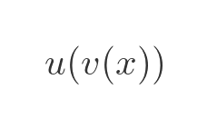
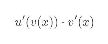
The chain rule allows us to calculate the first derivative of that function. It is:

Proof when x = 1

When x = 1 we get this integral, as we saw earlier (recall that we have moved the negative sign outside the integral):

There is a standard trick that is used to integrate the ln function using integration by parts. We set f equal to the ln function, and make g' equal 1:

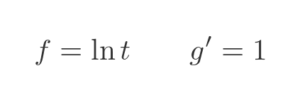
The derivative of ln t and the integral of 1 are both standard results:

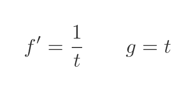
We put all these terms into the integration by parts formula (remembering the negative sign from earlier), and simplify:

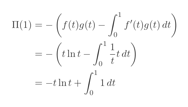
Evaluating the definite integral gives:

As we noted before, the term in t ln t vanishes at 0 and 1, so we have:

Proof when x = 2

In the second step, we use a different function, the square of the log function. This time the negative disappears because we are squaring the integrand:

This gives us the following terms, using the same trick as before, g' = 1:

We can find the derivative of f using the chain rule, defined above, where u and v are:

Which means u' and v' are:

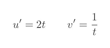
As we noted earlier, the all-important factor of 2 arises because the ln term is squared, which means u is the square function, which in turn means u' has a factor of 2. Plugging these into the chain rule formula gives:

So here are f' and g that we need for the integration by parts:

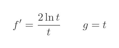
We can calculate the integral as before:

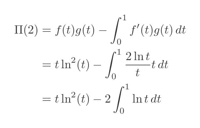
Notice that the integral term (including the negative sign) is equal to 2 times Π(1):

So, once again removing the term involving t and ln t, we have:

Which proves the pi function for 2.

We won't take this any further here, but using the same techniques, we can show that:

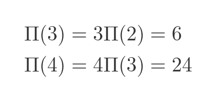
And so on.