Numerical integration

In mathematics, integration is the opposite process to differentiation. Where differentiation can be used to find the rate of change of a curve, integration is commonly used to find the area under a curve, or the volume under a surface, or the equivalent in higher dimensions. Integration is also used to solve differential equations, amongst many other applications.

We know how to differentiate many different types of mathematical functions because we can often find derivatives from first principles. We can't generally integrate a function from first principles, so we can usually only find the integral of a function by applying what we know about derivatives. For example, if we know that differentiating f(x) results in g(x), we can determine (subject to certain conditions) that the integral of g(x) is f(x).

A consequence of this is that there are many functions that we cannot integrate analytically.

But sometimes we only need to know the approximate value of a definite integral (that is, the area under a curve between two points a and b). Numerical methods provide ways to calculate approximate integrals, often accurate to many significant figures, that are fine for most practical purposes.

This article will look at some of those methods:

• Rectangular approximations
• Trapezium rule
• Simpson's rule
• Monte Carlo methods
• Integration by series expansion

Example

Here is a function f(x), and we wish to find an approximate value for the definite integral between x-values a and b:

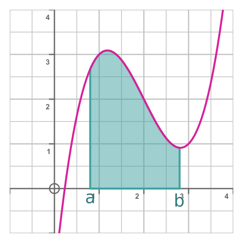
If we cannot integrate f(x) directly, we must look for an alternative solution. If we think of the problem in terms of calculating the approximate area under the curve, them we might consider a geoemetric approach. We will look at several approaches that can be used to calculate the area under almost any curve, perhaps to 6 signficant figures or better.

The function shown is:

Of course, since this is a polynomial we can find its integral fairly easily, although for this article we will pretend we can't. The integral (ignoring the constant of integration) is:

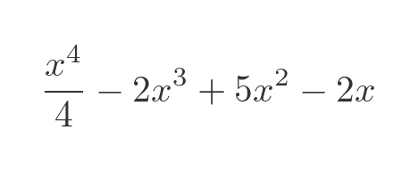
Before we go back to pretending we don't know this result, we will note that the integral between the range shown (0.8 to 2.8) is exactly 4.384. We can compare our approximate results to this exact value to see how well the approximations work.

Rectangular approximation

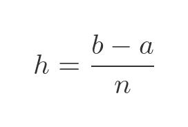
One possible approximation is to divide the area into n rectangles. We start by dividing the range a to b into n slices, each of width h:

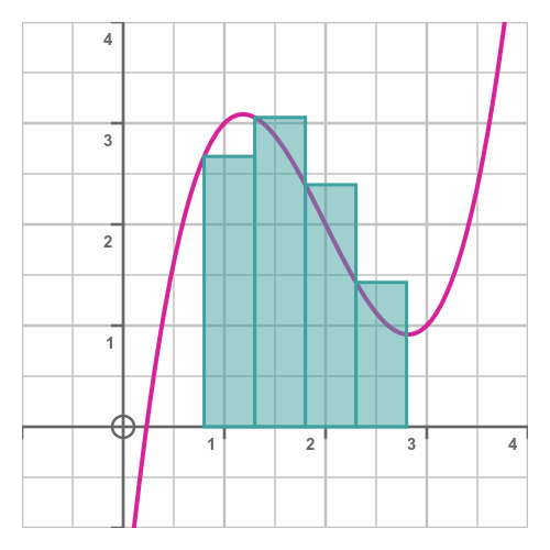
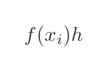
We have labelled the x-axis with n + 1 equally spaced values, where x0 is the start value, a, and xn is the end value, b. Now we can draw rectangles to approximate the area under the curve. Rectangle i starts at position xi, with height f(xi) and width h:

The width h is simply the distance from a to b, divided by n:

The area of rectangle i is given by:

We can see from the image that, provided the function behaves reasonably smoothly over the range, the total area of all the rectangles will be approximately equal to the area under the curve. To illustrate the technique, we have only used four slices, so it is easy to see how the area of the slices differs from the area under the curve. But a computer would easily be able to calculate thousands or even millions of slices in a very short time, giving quite an accurate estimate of the true area (see below).

The total area of all the rectangles is:

We have labelled this the lrect area because it is formed from rectangles whose height is given by the value of the function at the left-hand bound of the rectangle.

How accurate is this approximation? Recall that the exact area is 4.384. The approximate results (to four decimal places) are:

• 4 slices: 4.7740
• 1000 slices: 4.3857

Not surprisingly, 4 slices give a fairly inaccurate result. 1000 slices is correct to almost three dp.

Alternative rectangle form

We could draw the rectangles in a slightly different way, like this:

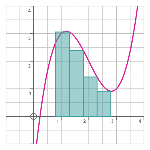
This time the height of each rectangle is given by the value of the function at the right-hand bound of the rectangle, so we will call this the rrect area. It is calculated using this slightly different formula:

All we have done here is let the summation count from 1 to n, rather than 0 to n - 1 as before. This means that the first rectangle has a height of f(x1) rather than f(x0), and similar for all the other terms.

The new results are:

• 4 slices: 3.8940
• 1000 slices: 4.3822

The lrect area and the rrect area are always likely to be slightly different. Depending on the curve and the position of the endpoints, one or the other might be more accurate. However, there is a simple technique for getting the best of both worlds, as we will see next.

Trapezium rule

Rather than trying to model the area using rectangles, we could try using trapezium shapes, like this:

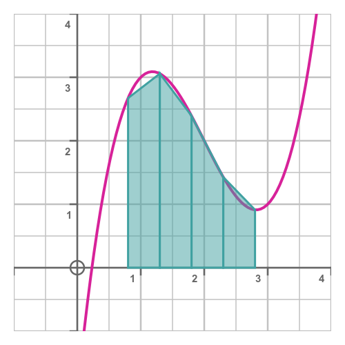
This looks like it fits the curve much more accurately, so we would expect a more accurate result.

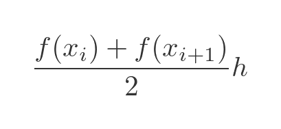
How is this calculated? Well, the area of a trapezium is the width multiplied by the average height, so the area of trapezium i is given by:

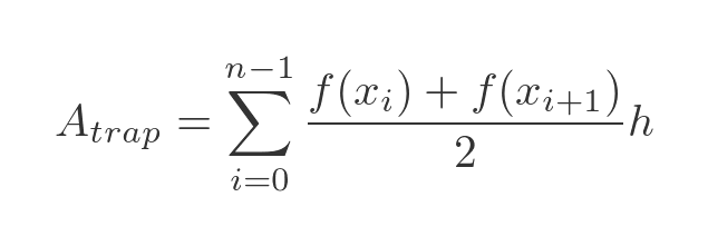
The total area is:

If we expand out the sum, we get this:

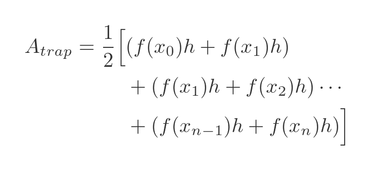
The thing to notice here is that term 0 only appears once, and term n only appears once. But every other term appears twice. So we can gather terms 1 to n - 1 in a new summation, and because each term appears twice, the factor of a half cancels out. Giving us this:

This is almost exactly the same as the formula for the rectangular approximation, except for a couple of extra terms. So calculating the trapezium approximation is not significantly more difficult than the rectangular approximation.

The results for the trapezium are:

• 4 slices: 4.3340
• 1000 slices: 4.3839992

The 4-slice result is more accurate, although still not good. But with 1000 slices, our result is correct to about six dp. Of course, that could still vary for different functions. But it is a very good improvement considering that the calculation only involves a tiny amount of extra work.

Another way of viewing the trapezium rule

Just as an aside, there is another interesting take on the trapezium rule.

We previously calculated the rectangular approximation using the left bound, lrect, and also using the right bound, rrect. It turns out that the trapezium approximation is simply the average of those two values:

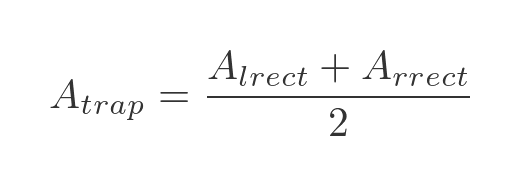
It is easy to see why this is true by considering lrect and rrect as summations:

If we expand out the two sums, then clearly term 0 only exists in the first sum, term n only exists in the second sum, but terms 1 to n - 1 exist in both sums. This matches the previous expression for the trapezium approximation:

Which proves the result above.

Simpson's rule

Simpson's rule takes the trapezium rule one step further. With the trapezium rule, we fit a straight line between each pair of points. Simpson's rule takes three points at a time and fits a quadratic curve to those three points. This is illustrated here:

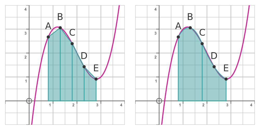
The LHS shows the trapezium rule, exactly as we saw earlier. We have points, A to E. We approximate the area by drawing straight lines from A to B, and from B to C, etc, and finding the areas of the trapeziums.

The RHS shows Simpson's rule. We have the same points, A to E, but this time we take three points at a time. Looking at the first three points, we draw a quadratic curve that passes through the points A, B and C. We then find the area under the quadratic curve - this is a standard integral. We then repeat this process starting from the last point, C, fitting a quadratic to C, D and E.

In our example, we only have two slices, but if we had more slices we would continue this process with points E, F and G, and so on.

As the diagram illustrates, a quadratic curve will usually fit the curve more accurately than two straight-line sections, so the result will usually be more accurate. So we can find a better approximation to the area without needing to calculate more points on the curve.

But isn't the process a lot more complicated? We need to fit a quadratic curve to three points, which involves solving three simultaneous equations. We then have to find the area under the quadratic curve. Doesn't this all take time?

Well, as you may have guessed from the rhetorical question, no it doesn't take significantly longer than the trapezium or rectangle cases. We are only interested in finding the area under all the curves, and while we do have to fit the curves and integrate the results, the final equation is pretty simple. That is the beauty of Simpson's rule. The derivation is slightly too long to include here, but it is quite satisfying, so it will probably form a future article.

The final equation is:

Since we pair up the slices, we need n to be even to use Simpson's rule. We then add up all the f(x) values, each multiplied by a particular number:

• Points 0 and n are multiplied by 1.
• Of the remaining points, the odd numbered points are multiplied by 4
• And the even numbered points are multiplied by 2.

The sum is then multiplied by the slice width h and divided by 3.

This technique is considerably more accurate than the trapezium rule. On our test function, the accuracy is better than 6 dp even with only 30 slices! However, this might vary for different types of function.

Monte Carlo method

A Monte Carlo method is a probabilistic method for solving a problem numerically. Essentially we define a rectangular area completely enclosing the area we wish to integrate. We then generate a set of random points within that rectangular area, like this:

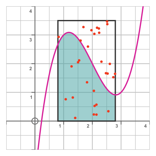
Each red dot represents a random point. There are 30 points, and 13 of them are within the curve whose area we are trying to estimate.

Based on that, we can estimate that the area under the curve is equal to 13/30 of the total area of the rectangle.

Since the rectangle has width 2 and height 3.5, its area is 7.

Therefore, the area under the curve is estimated to be:

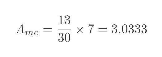
This is quite a long way off the true number. That is because it is based on 30 random trials, which is too small to give an accurate result.

Unfortunately, this method converges very slowly. Even a million random samples will only give about two decimal places of accuracy. The benefit of the Monte Carlo method is that it is a very simple algorithm to find an approximate answer, and it can be applied to a wide variety of problems.

Series expansion

This final technique works if we know how to approximate the function as a polynomial. The series will often be the Macalaurin expansion of the function we wish to integrate. A Maclaurin expansion is an infinite polynomial of the form:

In a Maclaurin expansion, the polynomial coefficients often decrease as the inverse factorial, so a good approximation can be found using a reasonably small number of terms.

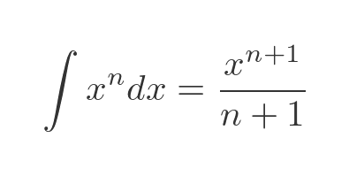
Once we know the Maclaurin expansion, it is easy to integrate it, using the standard integral of x to the power n for each term (ignoring the constant of integration):

As an example, we will apply this to the function:

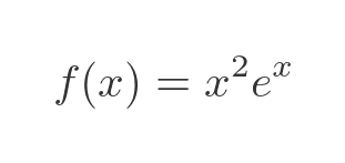
Now it is possible to integrate this analytically, using integration by parts, applied twice. We get this:

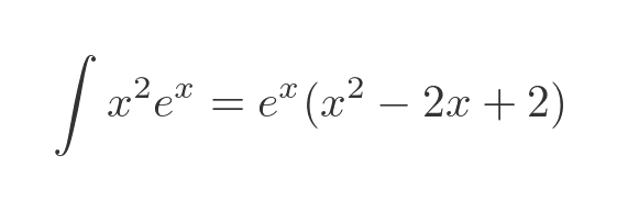
But again we will pretend that we can't do that. Instead, we will use the series expansion method. The Maclaurin expansion of the exponential function is a standard result:

Our function is the exponential function multiplied by x squared. We can find the series for our function by multiplying the result above by x squared:

The integral of our function is the sum of the integrals of each term:

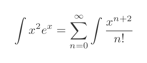
Applying the standard result for integrating x to the n (or n + 2 in this case) gives:

Integration by series expansion requires a bit of initial work to set up. But once that work is done, the integral can be calculated very accurately, and very quickly. Calculating ten or twenty terms on the series might give a result that is more accurate than the trapezium method with a million slices. This technique is well suited to situations where you might need to calculate the same integral with different limits, many times, and you need an accurate result.

See also

• Solving equations numerically
• Solving equations using interval bisection
• Solving equations using linear interpolation
• Solving equations using the Newton-Raphson method