Drawing Sierpinski triangles

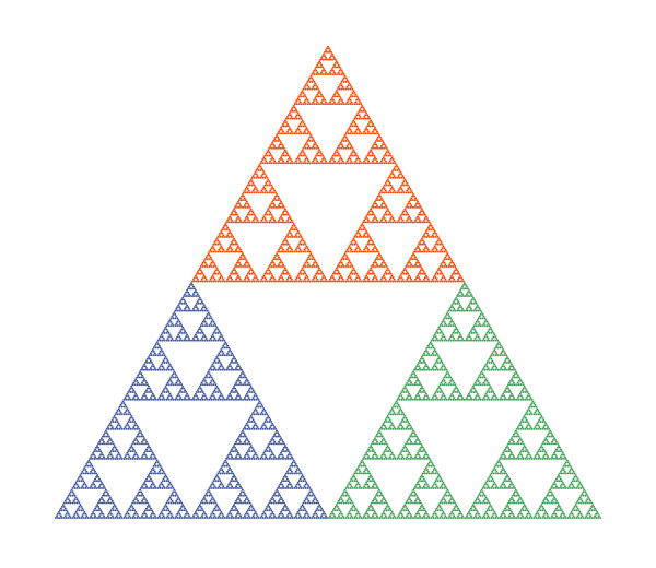
The Sierpinski triangle is a very well-known self-similar fractal.

There are many different ways to draw this fractal. We will look at some of the methods here. We won't go into a great deal of detail about each method, they will be covered in other articles.

Triangle replacement

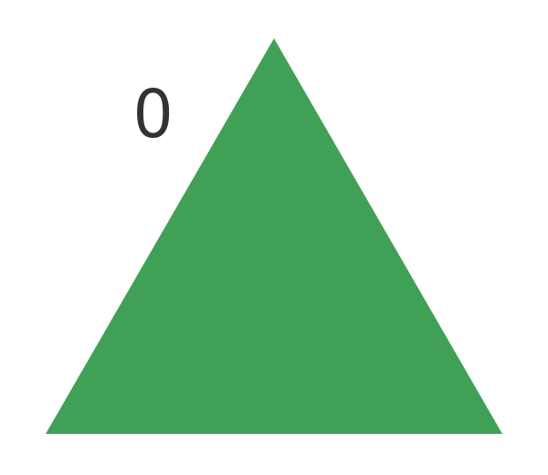
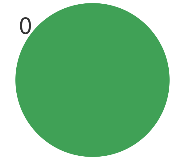
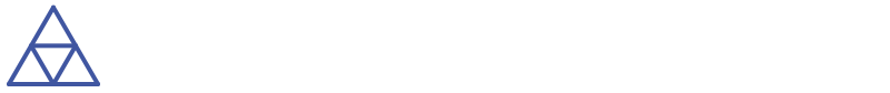
The most obvious way to draw a Sierpinski triangle is by triangle replacement. Starting with a single triangle:

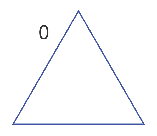
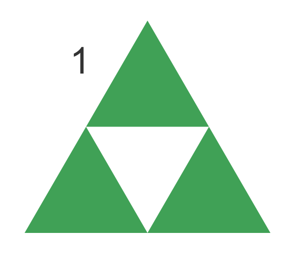
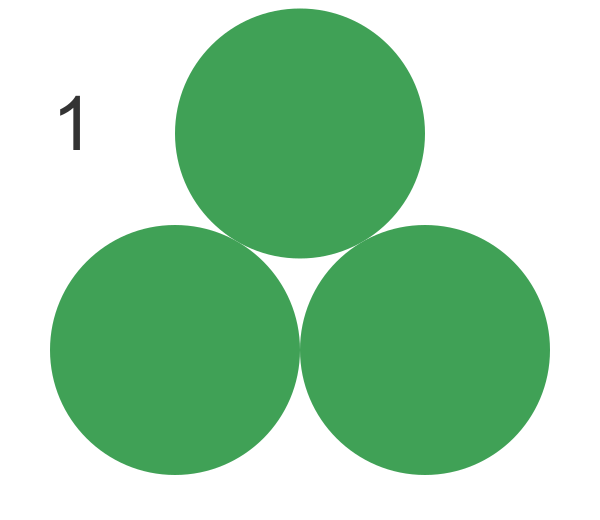
We have marked this as level 0, the initial starting triangle. Now we can replace this big triangle with three smaller triangles, one at the top, one at the bottom left, and one at the bottom right. We call this level 1:

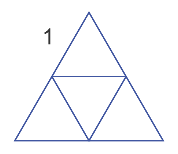
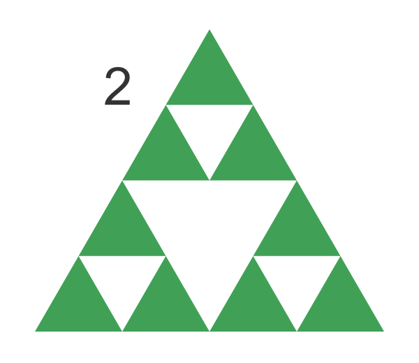
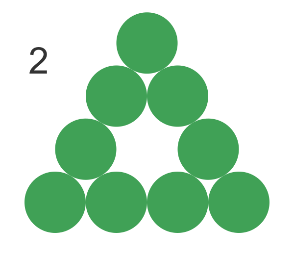
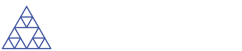
For the next step, we replace each of the three smaller triangles with three even smaller triangles. Notice that the central triangular area is a "hole" so it is left as it is. We call this level 2:

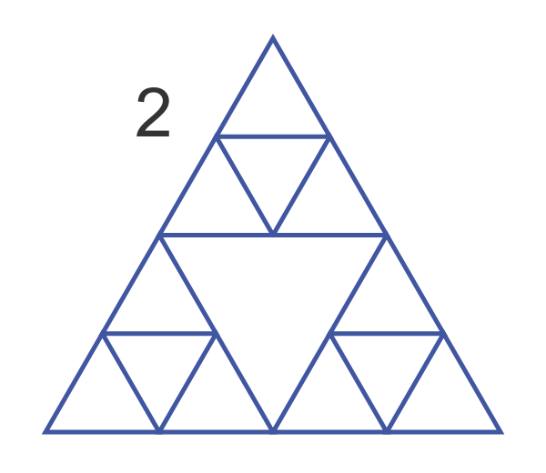
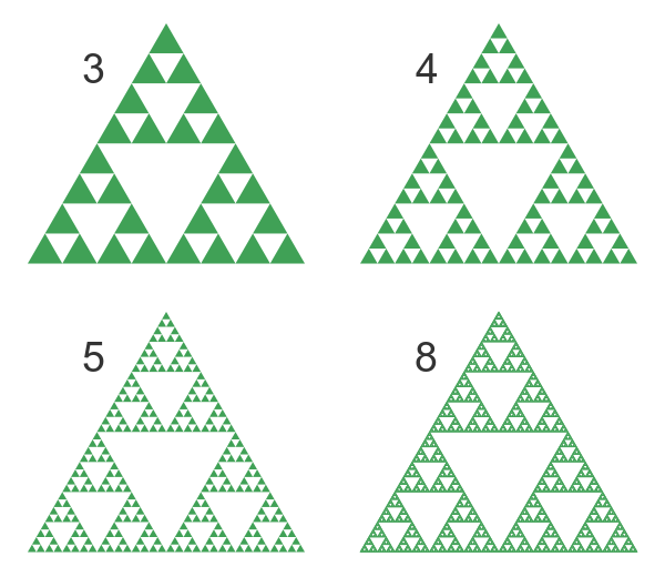
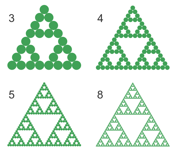
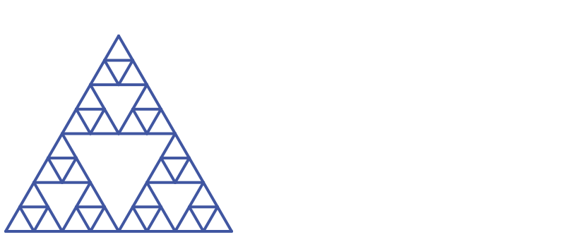
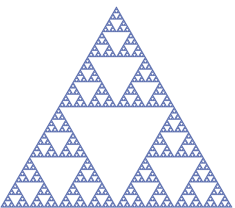
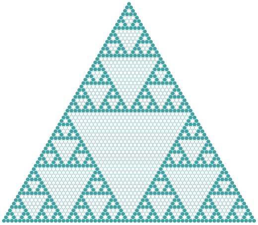
We repeat this again for levels 3, 4, and 5. By level 8 the triangles are too small to see, so the shape looks like the familiar Sierpinski triangle:

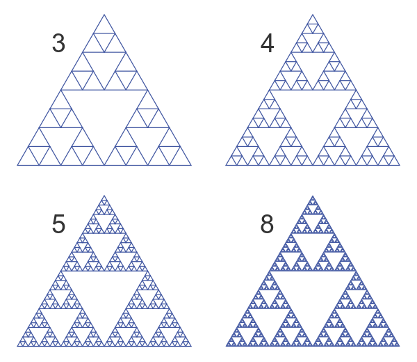
For a real Sierpinski triangle, this process must be repeated forever, so that there are infinitely many triangles that are infinitesimally small. But for the purpose of drawing the triangle, as soon as the triangles are too small to see the drawing is accurate enough.

Drawing a Sierpinski triangle by hand

There is a similar method that is quite useful if you ever want to hand-draw an approximate Sierpinski triangle. Start by drawing the large triangle. Then mark the midpoints of each side of the triangle, and use them to draw an inner triangle:

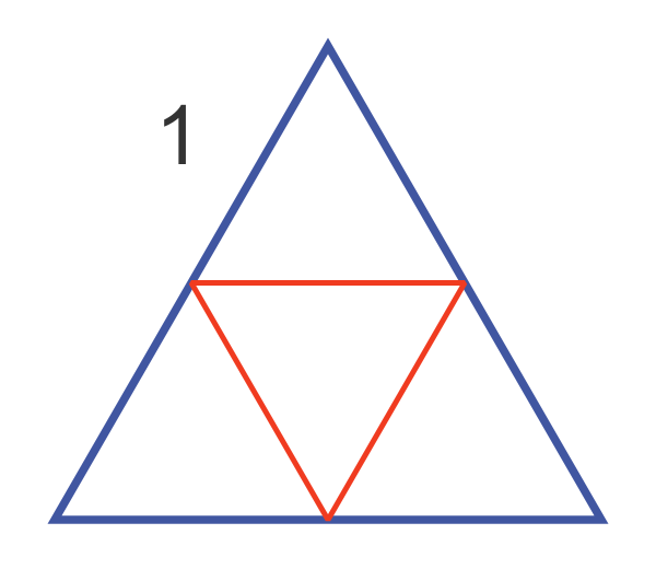
We have drawn the main triangle in blue and the second triangle in red, for clarity, but if you are drawing the triangle you will probably want to draw it all in the same colour. The drawing about is level 1.

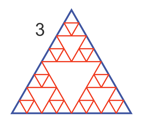
To draw level 2, we mark the midpoints of each side of the small triangles, and use them to draw an even smaller inner triangle:

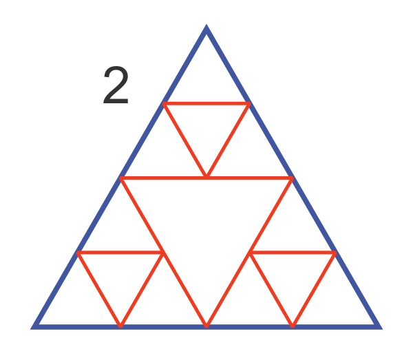
This can be repeated to draw level 3, and depending on your patience levels 4 and beyond:

Cutting holes

A different approach is to start with a filled triangle and cut holes in it. Here is level 0:

To create level 1, we cut a triangular hole in the main triangle, leaving three small triangles:

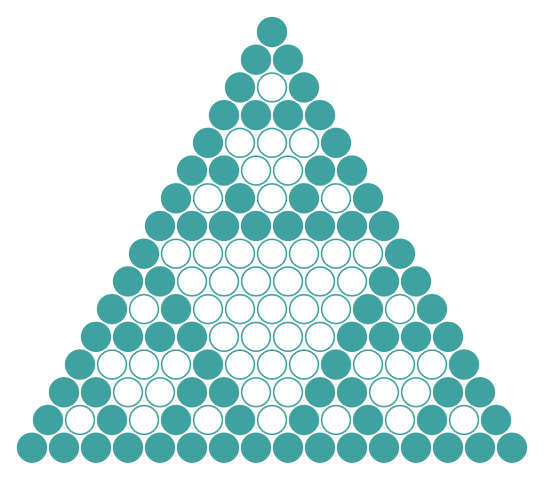
For level 2 we cut a triangular hole in each of the three small triangles:

We can keep doing this. Although this triangle is not the same as the triangle replacement method, the more levels we apply, the closer it gets. By the time we reach level 8, we can no longer see the small triangles so it looks very similar to the other method:

Collage theorem

This is not, in itself, a way of drawing Sierpinski triangles, it is more of an interesting fact. But it leads to a couple of ways of drawing the triangle.

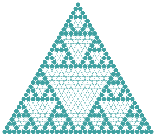
Here is a Sierpinski triangle where the three sub-triangles have each been drawn in a different colour:

Here is the interesting fact - each of the three different coloured triangles is an exact copy of the original triangle.

In other words, if you take three copies, A, B, and C of the original triangle and you:

• Shrink A by a factor of two.
• Shrink B by a factor of two and shift it by half a unit to the left.
• Shrink C by a factor of two and shift it by half a unit upwards at an angle of 60 degrees.

The triangles A, B, and C will make an exact copy of the original triangle.

Another, perhaps more interesting fact is that the Sierpinski triangle is the only shape that will map onto itself exactly using those three particular transforms.

Other self-similar fractals - for example, the Koch curve or the Cantor set - have the same property, but of course the actual transforms are different. The collage theorem tells us that if we know the set of transforms we can draw the fractal, and it provides us with two different ways to do this, which we will look at next.

Collage theorem deterministic algorithm

Let's assume we have a self-similar fractal, such as a Sierpinski triangle. Let's also assume we know the set of transforms T that define the fractal. For a Sierpinski triangle the set T will contain the three transforms described above.

The deterministic algorithm works as follows:

1. Choose a suitable starting point, such as (0, 0).
2. Apply each of the transforms in T to the starting point. This will create a set of points P.
3. Apply each of the transform in T to each point in P. This will create a new set of points P.
4. Repeat from step 3 n times.
5. Plot a dot at each point in P.

As an example, we will start with one circle at (0, 0). This is the start step, 0:

We have used circles but it really doesn't matter what shape you use. It will eventually be too small to see. Next, we apply the three Sierpinski triangle transforms to the large dot:

This creates three smaller dots (half the previous size) which have been positioned by the transforms into the places normally occupied by the three sub-triangles.

Now we apply the same three transforms to each of the three dots. This creates nine even smaller dots:

If we apply this three, four, or five times we get an increasing number of smaller dots:

By iteration eight, the dots are too small to see, and we have a version of the Sierpinski triangle.

Collage theorem chaos algorithm

There is a completely different method of drawing a Sierpinski triangle from its transforms. It works like this:

1. Choose a starting point p, somewhere inside the main triangle.
2. Pick one of the three transforms at random.
3. Apply the chosen transform to the point p. The transformed point becomes the new point p.
4. Put a dot at the new point p.
5. Repeat from step 2, n times.

When we use this method, since we are continuously transforming the current point by transforms selected at random, the points initially appear to be scattered all over the place. This is what it looks like after 100 iterations:

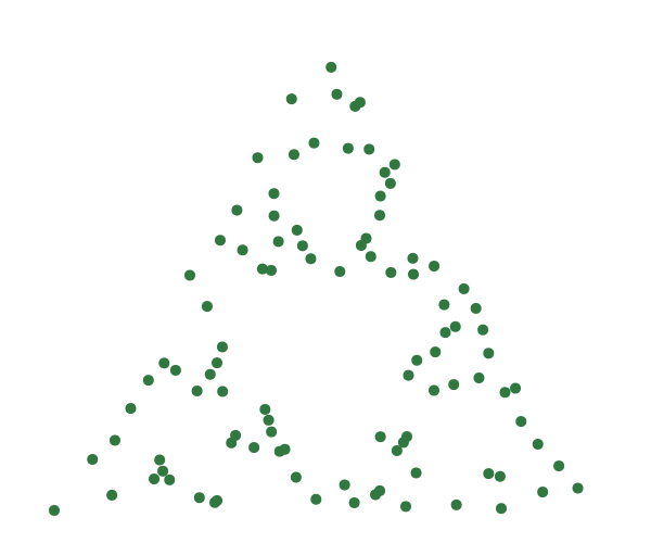
This gives a vague hint of the true shape of the final triangle. If we increase the number of iterations to 1000, and also make the dot size smaller, we get something that is a little better:

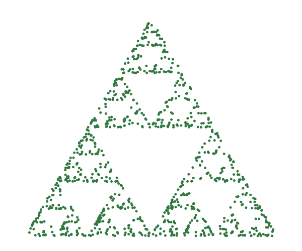
But in order to get something that looks like a good approximation to the Sierpinski triangle, we need 100,000 iterations (and again an even smaller dot size):

It might seem that the chaos method requires far more iterations than the deterministic method, but bear in mind that each iteration of the chaos method adds one point to the image, whereas each iteration of the deterministic method multiplies the number of points by three.

So ten iterations of the chaos method create three to the power ten points, which is about 60,000 points. So the methods aren't so different.

L system triangles

An L system is a grammar-based system that "grows" self-similar fractals. It was originally invented to simulate biological processes, but it can be used to draw a Sierpinski triangle too.

We start by defining an alphabet for our simulation. For a Sierpinski triangle, we can use an alphabet of four symbols. We will use "F", "G", "+" and "-".

We also define a set of rules. On each pass through the algorithm, we replace each symbol with a string of new symbols:

• "F" is replaced with "F-G+F+G-F".
• "G" is replaced with "GG".
• "+" is replaced with "+" (we say "+" is a constant).
• "-" is replaced with "-" ("-" is also a constant).

We start with an initial string, called the axiom, which has the value "F-G-G".

When we apply these rules to the initial string, replacing each "F" and "G" with the new value and leaving the constant symbols unchanged, we get:

• "F-G+F+G-F-GG-GG"

The next step is to define the set of drawing operations for each symbol. We will base this on turtle graphics and define the following operations:

• "F" moves the turtle forward by one unit, drawing a line as it goes.
• "G" also moves the turtle forward by one unit, drawing a line as it goes.
• "+" turns the turtle left by 60 degrees.
• "-" turns the turtle right by 60 degrees.

If we apply these rules to the string above, we draw this shape:

Applying the rule again yields this string:

"F-G+F+G-F-GG+F-G+F+G-F+GG-F-G+F+G-F-GGGG+F-G+F+G-F-GG+F-G+F+G-F+GG-F-G+F+G-F+GGGG-F-G+F+G-F-GG+F-G+F+G-F+GG-F-G+F+G-F-GGGGGGGG-GGGGGGGG"

And this triangle:

This image is similar to the second-level image of the first triangle replacement method but with an important difference. In the previous image, the overall triangle remained the same size, and additional detail was added in the form of smaller and smaller triangles within it. In an L system, the overall shape gets bigger on each pass. The smallest triangles are still the same size as before.

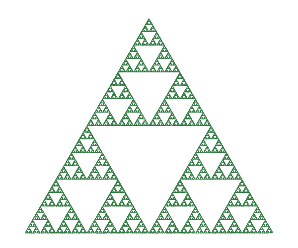
This continues when we go to the third level:

Here is the shape after 8 iterations. The previous triangles were all drawn to the same scale, but this triangle has been scaled down by a factor of 13 because otherwise it would be far too big to fit the page.

In this system, a Sierpinski triangle with an infinite level of detail would be infinitely large.

Arrowhead Sierpinski triangle

We can also make a Sierpinski triangle using an arrowhead shape. In this method, the entire triangle is made from a single line that never splits or intersects itself. We can create this using an L system with slightly different rules (see below).

Here is the first level:

There are 9 lines in this arrowhead shape. For the second level, we replace each line in the original shape with a complete new arrowhead:

After a couple more iterations (and scaled-down) we can see the Sierpinski triangle shape starting to form, but notice that the whole shape is just a single line (with lots of twists and turns):

Eventually, we end up with a shape that looks just like the triangle created by other methods. It is still all one line, but in many places, the line gets so close to itself that it appears to intersect.

If you are interested, the L system rules for drawing this shape are:

• "F" is replaced with "G-F-G".
• "G" is replaced with "F+G+F".
• "+" and "-" are constants as before.

With everything else remaining the same.

Pascal's triangle

You will probably be familiar with Pascal's triangle:

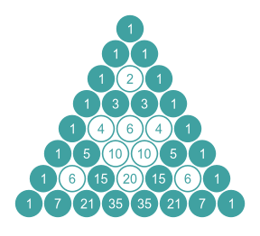
In this triangle, the elements on the left and right edges are all set to one. Each of the elements in the middle is formed from the sum of the two elements above it. In the diagram above we have shaded the elements that are odd numbers.

Let's add a few more rows:

And more, again with all the odd numbers shaded:

And more:

This is definitely a Sierpinski triangle! Like the L system example, this triangle gets bigger as we add more levels, so it needs to be scaled down each time.

It is no coincidence that the odd numbers in Pascal's triangle form a Sierpinski triangle, but that is a topic for another article.

Cellular automaton

A cellular automaton is a collection of square "cells" that each contains a number.

At regular intervals, each cell changes from its current value to its next value. The next value is determined by the current state of itself and its neighbours, according to a fixed rule.

We will look at this system:

• There are nine cells, in a straight line, so each cell has two neighbours (except the cells at the end, which only have one neighbour).
• Each cell can only have a value of 1 or 0.
• The next value of a cell will be 1 if exactly one of its neighbours has a current value of 1, otherwise it will be 0.

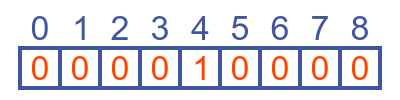
Here is the initial value of the system, with just the centre cell set to 1:

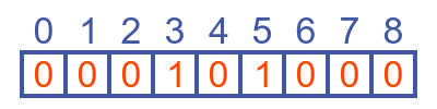
In this case, most of the cells have neighbours with a value of 0, so their next value will be 0. However, cells 3 and 5 both have a single neighbour with a value of 1, so their next value will be 1. Notice that although cell 4 has a current value of 1, it has a next value of 0 because both its neighbours are currently zero:

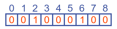
Now three cells have neighbours with value 1. Cell 2 has one neighbour with a value of 1, so its next value is 1. Cell 4 has two neighbours with a value of 1, so its next value is 0. Cell 4 has one neighbour with a value of 1, so its next value is 1.

If we continue these calculations, we can create a chart where each row represents the next step. Here is the result for the first 32 steps:

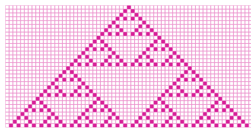
Once again, we see the familiar shape of a Sierpinski triangle!

See also

• Bifurcation and chaos
• Cantor set
• Koch snowflake