L system Koch curve

L Systems were developed by Aristid Lindenmayer, a biologist, to model plant growth. But L Systems can also be used to describe fractals. And, not surprisingly given their origins, they are very good at creating natural-looking fractals such as tree and fern-like structures.

An L System is primarily a way of manipulating strings of characters. It starts with an initial string and applies a set of rules repeatedly to generate more complex strings.

Although L Systems work on character strings, we can convert them into images by treating each character in the string as a drawing instruction.

A simple L System - algae

To define an L System, we first define the alphabet (ie set of symbols we will use in the system) it uses. To keep things simple, in this example, we will use an alphabet that consists of just two letters, A and B.

We then have to define a set of rules. The rules are used to transform a string of symbols into a different string. In an L System, there is one rule for each symbol, and it determines how that symbol is transformed. The two rules we will use are:

A becomes B
B becomes BA

Finally, we must define our initial string, sometimes called the axiom. In this case, we will start with the string A.

Iteration 1

On each iteration, we take each character in the current string and apply the rules to create a new string.

Our current string is A, so we apply the rule A becomes B, giving us a new string B.

Iteration 2

Our current string is now B, so we apply the rule B becomes BA, giving us a new string BA.

Iteration 3

For the third iteration, the current string is now BA.

We apply the rules to each character in the string, and concatenate the results:

• The first character, B becomes BA.
• The second character A becomes B.

When we join these together we form the string BAB.

Iteration 4

Our current string is now BAB, so:

• The first character, B becomes BA.
• The second character A becomes B.
• The third character, B becomes BA.

Concatenating these strings gives BABBA.

If we continue this, the next string will be BABBABAB, and then BABBABABBABBA and so on.

This system is meant to give a very crude model of how algae grow. One thing you might notice is that the lengths of the strings are 1, 1, 2, 3, 5, 8, 13 ... the Fibonacci series. This shouldn't be too surprising because, of course, the Fibonacci series is often observed in nature.

Algae in Python

Before attempting to draw anything, let's implement this system as a simple Python program:

AXIOM = 'A'
RULES = { 'A' : 'B',
          'B' : 'BA'}
ITERATIONS = 6


def lsystem(start, rules):
    out = ''
    for c in start:
        s = rules[c]
        out += s

    return out


s = AXIOM
print(s)
for i in range(ITERATIONS):
    s = lsystem(s, RULES)
    print(s)

We have defined our AXIOM (the initial string), and our set of RULES. The rules are implemented as a Python dictionary. For each input symbol, the dictionary supplies the string that the symbol will be replaced with.

The lsystem function accepts parameters start (the string to be converted) and rules (the rules dictionary). It loops over every character in the string, converting it via the rules dictionary, and adding it to the end of the output string.

Finally, the main loop iterates 6 times, printing the output string at each stage.

L System for a square Koch curve

Now we will see how to create a drawing with an L System. We will draw a classic fractal, the square Koch curve.

The L System works in the same way as before - we have an alphabet of characters, a set of rules, and an axiom (the initial string).

But to create a drawing, we must do one extra thing. We must associate each letter in the alphabet with a specific drawing operation. But bear in mind that the drawing operations are an extra layer on top of the normal L System. The L System itself works in exactly the same way as before, with no knowledge of the drawing operations. We then apply the drawing operations to the result created by the L System.

For the Koch curve, we will use an alphabet of three characters: F, +, and -.

Our rules are:

F becomes F+F-F-F+F
+ becomes +
- becomes -

Note that symbols like + or -, which are always replaced with themselves, are called constants in an L System.

Our axiom is F.

What about our drawing operations? We will use a simple turtle graphics model, where an imaginary "turtle" moves around the page, drawing lines as it goes. The rules are:

• Initially the turtle is at position (0, 0), pointing right (ie along the positive x-axis).
• F makes the turtle move forward by a 1 unit, drawing a line as it goes.
• + makes the turtle turn to the left by 90 degrees, without moving.
• - makes the turtle turn to the right by 90 degrees, without moving.

Iteration 1

After one iteration, the initial F will be replaced with F+F-F-F+F. This string can be interpreted as:

• Forward 1 unit
• Left 90 degrees
• Forward 1 unit
• Right 90 degrees
• Forward 1 unit
• Right 90 degrees
• Forward 1 unit
• Left 90 degrees
• Forward 1 unit

This draws a shape like this:

Starting from the leftmost point of the figures, if you follow the drawing operations above, you should be able to see how this figure is drawn.

Iteration 2

On the second iteration, we start with the previous string F+F-F-F+F.

Each F in this string is replaced with F+F-F-F+F, giving:

F+F-F-F+F+F+F-F-F+F-F+F-F-F+F-F+F-F-F+F+F+F-F-F+F

This is the result when we interpret this string as drawing instructions:

We can draw this curve by simply following the drawing instructions above. But we would like to understand this curve a little better.

The string F+F-F-F+F represents the curve we drew in iteration 1. This same string appears several times in iteration 2. Let's replace this string with curve1:

curve1+curve1-curve1-curve1+curve1

So what we are doing here is drawing curve1 (the curve from iteration 1). Then from the end of that curve, we turn left and draw curve1 again. Then we turn right and draw it again, right and draw it again, and finally left and draw it a fifth time.

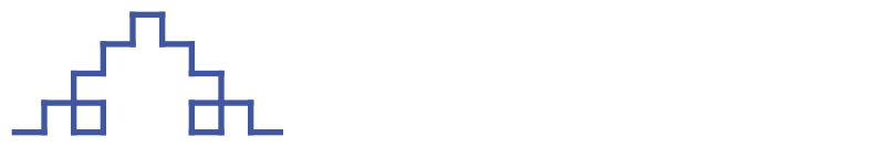
It is worth understanding why this happens. Here is iteration 1, but with each line (each F) drawn in a different colour (black, yellow, magenta, green, orange):

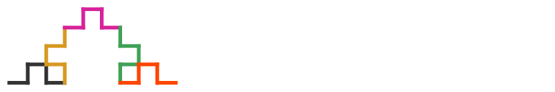
On iteration 2, each of those lines "grows" into a shape. Here is iteration 2 with each section coloured according to the line that generates it:

The curve gets bigger on each iteration, in fact, it gets three times wider each time. But this growth occurs because each part of the previous curve grows. This is intended to model the way plants grow.

There are various other ways to draw the Koch curve but most of them keep the size of the shape constant and incrementally add more detail. L Systems don't work that way.

The other thing to notice is that the string contains a full description of the curve. The drawing code just needs to follow the drawing instructions, one after another. The recursive nature of the shape is encoded into the string itself.

Iteration 3

For iteration 3, we repeat the same procedure. This generates quite a long string:

F+F-F-F+F+F+F-F-F+F-F+F-F-F+F-F+F-F-F+F+F+F-F-F+F+
F+F-F-F+F+F+F-F-F+F-F+F-F-F+F-F+F-F-F+F+F+F-F-F+F-
F+F-F-F+F+F+F-F-F+F-F+F-F-F+F-F+F-F-F+F+F+F-F-F+F-
F+F-F-F+F+F+F-F-F+F-F+F-F-F+F-F+F-F-F+F+F+F-F-F+F+
F+F-F-F+F+F+F-F-F+F-F+F-F-F+F-F+F-F-F+F+F+F-F-F+F

This can be simplified if we express it in terms of the previous curve, curve2:

curve2+curve2-curve2-curve2+curve2

So in effect, we are taking the five versions of the previous curve and laying them out in the shape of the first iteration. But remember that the growth is actually caused by each F in the previous iteration being replaced by F+F-F-F+F.

The final curve looks like this:

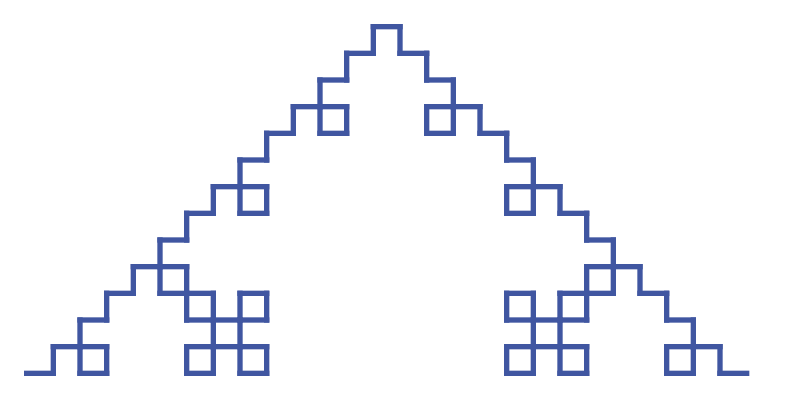
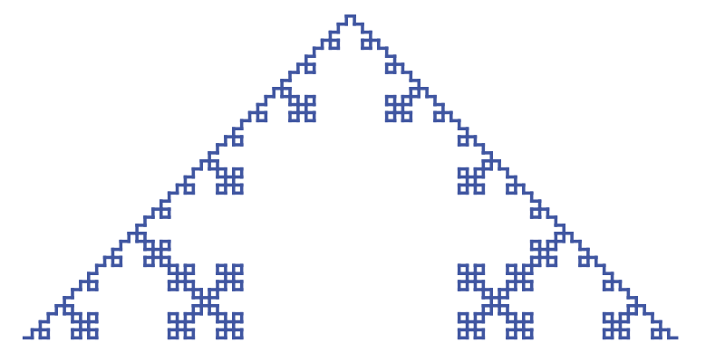
Iteration 4

Iteration 4 repeats the same process. By now the string is getting rather long, so we won't show it here. The curve itself is getting bigger too, as each iteration is three times wider than the last one.

So here is the curve for iteration 4, scaled down by a factor of 3 compared to the earlier curves:

Triangular Koch curve

Finally, we will show how changing the rules can result in a different fractal. In this case, the triangular Koch curve.

We will use an alphabet of three characters: F, +, -. The axiom is still F.

But the rules are slightly different, notice the double - symbol:

F becomes F+F--F+F
+ becomes +
- becomes -

The drawing instructions are slightly different too. The angle used for + and - is 60 degrees, rather than 90 degrees:

• F makes the turtle move forward by a 1 unit, drawing a line as it goes.
• + makes the turtle turn to the left by 60 degrees, without moving.
• - makes the turtle turn to the right by 60 degrees, without moving.

The first iteration is:

F+F--F+F

The figure created is:

The second iteration is:

F+F--F+F+F+F--F+F--F+F--F+F+F+F--F+F

Which creates this:

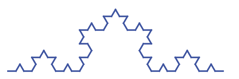
The third iteration is:

F+F--F+F+F+F--F+F--F+F--F+F+F+F--F+F+
F+F--F+F+F+F--F+F--F+F--F+F+F+F--F+F--
F+F--F+F+F+F--F+F--F+F--F+F+F+F--F+F+
F+F--F+F+F+F--F+F--F+F--F+F+F+F--F+F

Which creates this:

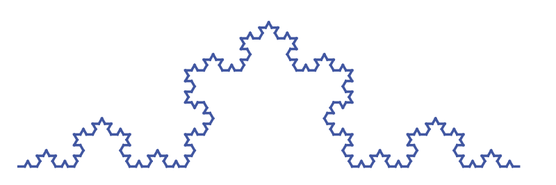
The fourth iteration creates this fractal, again scaled down by a factor of three because it has grown quite large:

See also

• L system trees and ferns