Bifurcation and chaos

In this article, we will look at a simple dynamical system representing constrained growth. For illustration, we will assume this represents the year-by-year population of rabbits in an environment where the amount of available food and space prevents the population from growing to an unlimited size.

As we will see, even a very simple model leads to complex and even chaotic behaviour in certain conditions.

Population model

We will use a very simple model of the rabbit population, year by year. We will start by assuming an unconstrained growth of the rabbit population is given by:

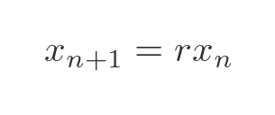
Where:

In this model, growth will continue forever. For example, if r is 2, the number of rabbits would double every year, forever, without limit.

This is clearly not realistic, the environment will normally place constraints on the population. For example, if the rabbits lived on a small island, it might be that there isn't enough food to support 1000 rabbits.

We can represent this by adding an extra term to our formula to represent constrained growth:

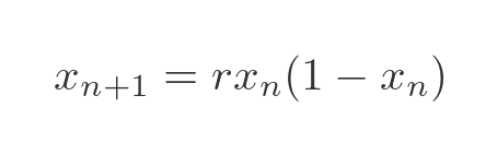
The extra term (1 - x) is a term that reduces to zero as x approaches 1. The value 1 represents the maximum number of rabbits. This acts as a scale factor between the equation and the number of rabbits. An x value of 0.5, for example, represents 500 rabbits (0.5 times 1000).

Interpreting the function

The formula above is a quadratic function in x. Here is what the function looks like as a graph (again, with an r value of 2):

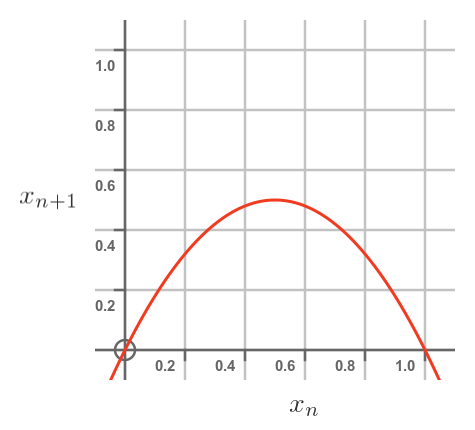
This graph tells us, given this year's population, how many rabbits there will be next year. The x-axis is the current population, and the y-axis is next year's population.

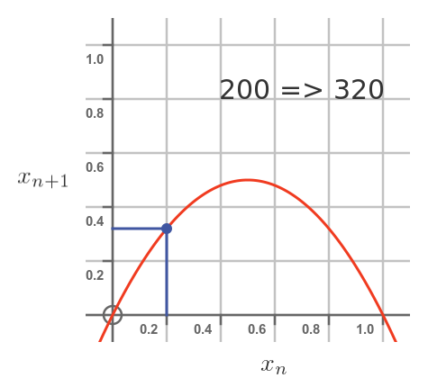
In the graph below, the current population is 0.2 (which equates to 200 rabbits). There is plenty of food and space, the rabbits will thrive, and if we read off the y-value it is 0.32. Our population of 200 will grow to 320:

Here is the graph again, but with a current population is 0.7. Food will be quite scarce, so not all the rabbits will survive and breed. There will actually be fewer rabbits next year than there were this year. Our 700 rabbits will dwindle to 420.

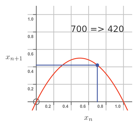
In summary, if there are less than 500 rabbits, there is plenty of food so the population will tend to grow. If there are more than 500 rabbits food will be a more scarce so the population will tend to fall.

Plotting the population over many generations

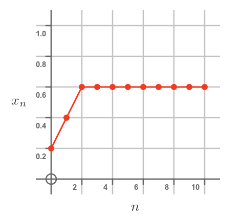
The previous graphs showed how the population changes between one year and the next. Now we will look at how the population changes over several years. This graph shows the population x for year n:

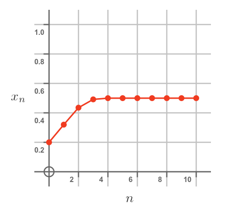
This initial population is 0.2. We can see that the population grows for the first few years, then eventually stabilises at 0.5. This means that when there are 500 rabbits, the birth rate will exactly match the death rate.

What happens if we start with a larger initial population, for example, 0.7 (like the earlier example)? Here is the graph:

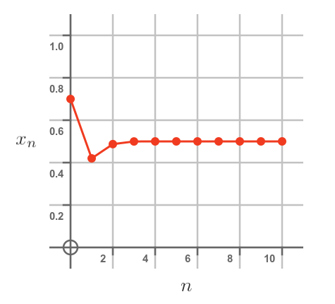
This time the population initially drops (as we saw before), but by the second year the population grows until, once again, it stabilises at 0.5. This shouldn't be surprising. The eventual stable population doesn't depend on how many rabbits there were in the first year. Of course, if the population was very small they might all die out, and if the population was very large they might all starve, so the population would vanish. But for any reasonable initial population, the final population will be 0.5.

So far we have only looked at a growth rate of 2. Here is what happens if we increase this to 2.5:

This time the population stabilises at 0.6 rather than 0.5. This makes sense. A higher population leads to a higher death rate, due to the 1 - x term in the formula. This is counteracted by the higher birth rate so a larger population can be sustained.

Effect of r on the population size

So now let's look at how the stable population varies with the growth rate r. Now we are no longer concerned with the initial population, or what happens in the first few years. We are only interested in the steady-state behaviour when the system stabilises.

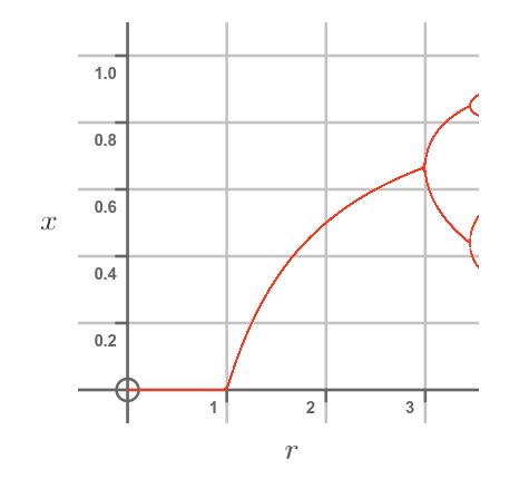
This graph shows the stable population x against r:

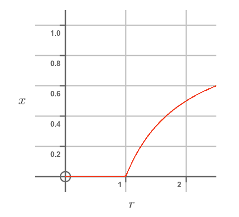
For growth rates of less than 1, the stable population is 0. That is simply because, if the number of rabbits born each year is smaller than the number lost, the population will eventually die out.

For growth rates of greater than 1, the population will grow to a stable level. As we saw earlier, the stable population is higher for higher growth rates.

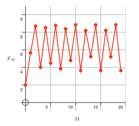
When r exceeds 3, something strange happens. Here is the population by year chart for r = 3.2:

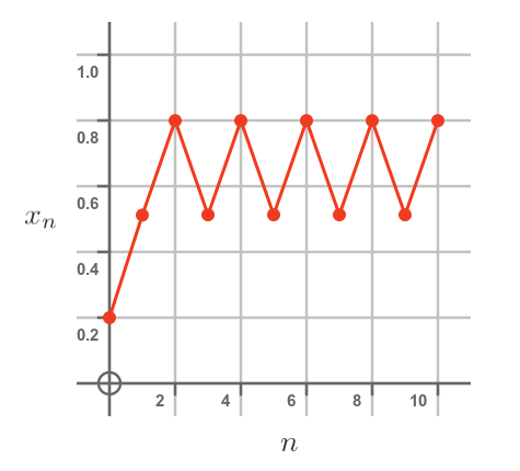
The population doesn't settle on a single value. Instead, it oscillates between 2 different values. And the oscillation doesn't fade away after a few years, it carries on forever.

One way to understand it is this. If we are in a year when the population is in its low cycle, then there will be plenty of food, so we would expect the population to be larger next year. But because the growth rate is so high, the population over-compensates and we end up with too many rabbits the following year. So the year after that, the number of rabbits reduces. But because it was so high before, it reduces by too much, so we end up at the same low value as the year before last.

The numbers flip between being too high and too low, never quite managing to stop in the middle.

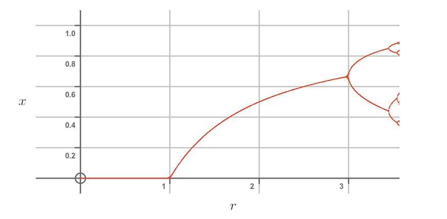
Here is the plot of x against r, extended to cover the range up to 3.2:

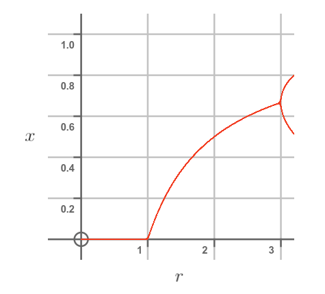
At r = 3 the plot splits into 2 values - this is called bifurcation. Initially, the split is very small, but as r increases the split gets wider.

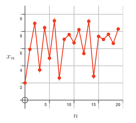
If we continue to increase r, then at a certain point we start to see another effect. Here is the population by year chart for r = 3.54:

The population still oscillates between high and low values, but there are 2 different high values and 2 different low values. The graph takes a little bit longer to stabilise, but it eventually enters a 4-year cycle between 4 different values. Here is the plot of x against r:

At a certain point, the graph bifurcates again, to give 4 different lines.

Chaotic behaviour

If we were to extend this graph further, it would soon split again. Each of the 4 lines would split, giving 8 lines. Then it would split again, giving 16 lines, and so on.

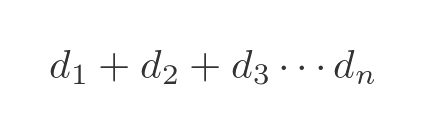
But we would also see that the splits get closer and closer together. Let's say that the distance from 0 to the first bifurcation is d1, the distance from the first bifurcation to the second bifurcation is d2, the distance from the second bifurcation to the third bifurcation is d3, and so on. The position of the nth bifurcation is the sum of all the distances between the first n bifurcations:

But as mentioned earlier, the values in the sequence d1, d2, d3 ... get progressively smaller. Sequences like that sometimes converge on a finite value. A familiar example of this is this sequence:

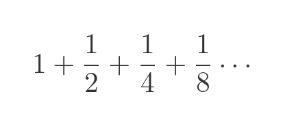
We know that this sequence converges on 2. As we add more and more terms, even as we approach an infinite number of terms, the sum will get closer and closer to 2, but never reach 2.

It can be shown that the bifurcation distance also converges. As n tends to infinity, the sum of the bifurcation distances converge to approximately 3.56995. This means that the bifurcations into 2, 4, 8, 16, and 32 strands, right up to an infinite number of strands, all happen before we reach that point (in much the same way that all the infinite number powers of a half fit into a finite range in the example above).

Here is a graph up to that point:

You can't see much of the detail. That is because each bifurcation gets closer and closer on the r axis, and also gets smaller and smaller on the x axis.

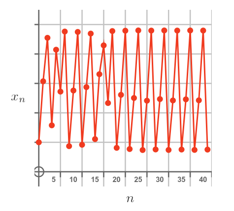
So what happens after this point? Well, the system becomes chaotic. Here is the population by year chart for r = 3.7 which is well into the chaotic region:

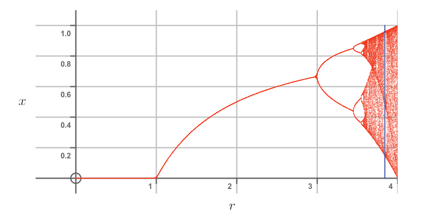
There is no repeating sequence here, the values are pseudo-random. Here is the plot of x against r for r up to 4:

Once we get past r = 3.56995, many values of x become possible, and the system flips between different values, chaotically.

Windows of order

If we look closely at the graph, we can see that even in the chaotic region, there is still structure. The most prominent feature is a gap at around 3.8284, marked with a blue line here:

These gaps are called windows of order. If we plot the population by year chart for r = 3.84 (inside the window region) we get this:

It takes a while to settle down, but eventually, it cycles through 3 different values. If we increase r slightly, This region bifurcates into 6 values, 12 values, and so on. This small region bifurcates an infinite number of times before becoming chaotic again. This, of course is typical fractal behaviour - small regions are similar, but not identical, to the whole fractal.

There are less prominent regions corresponding to other cycle lengths. In fact, if we choose any integer c, there will be some tiny region where the population has a cycle length c. And those regions are all contained in the region of r between 3 and 4.

Bifurcation in the real world

The effects described here are not critically dependent on the exact shape of the curve used in the logistic model. Some of the effects can be seen in real animal populations. For example, populations that alternate between low and high numbers in alternate years are sometimes observed.

The technique can be applied to other systems, for example fluid dynamics, where it can be used to explain certain types of turbulence in moving fluids.

See also

• Cantor set
• Koch snowflake
• Drawing Sierpinski triangles