The Lambert W function

In this article, we will look at the Lambert W function. This is a useful method of solving equations such as:

We will solve this equation shortly, but first, we will look at how and why standard functions like the Lambert W function come into being.

A nicer exponential problem

As a step along the way, we will look at a slightly different problem that turns out to have a nicer solution. We will solve this, and then use that solution to help with the original problem above. Here is the new problem, we need to find x where:

How would we solve this problem? Typically, we would solve for x, manipulating the equation to a form x equals some expression that doesn't involve x.

But in this case, we can't do that. There is nothing we can do to simplify the equation so that the left-hand side is just x and the right-hand side doesn't contain x.

Since we will be using this function later, let's call it G(x):

A potential solution

There is a typical way we often solve these types of problems, which is best illustrated using a slightly different (and more familiar) function. How do we solve this equation for x:

This is a similar format, we have an expression in x on the left and a constant on the right. We need to somehow simplify this so that the left-hand side is just x and the right-hand side doesn't contain x. Of course, we can solve this by taking the square root of both sides:

The reason we used the square root function is that it is the inverse of the x-squared function. The square root of x squared is simply x, because inverse functions essentially undo each other (care is sometimes required, see later). Applying this gives us:

So we have solved the equation.

Applying this to the original problem

We just solved an equation in x squared, using the inverse function, the square root of x. In general, we can do the same thing for any function f(x), provided it has an inverse function. For example, given this:

We can find x using the inverse of f(x):

In our original problem, we used the function as G(x):

We wanted to solve:

We now know that we can solve this equation, provided we know the inverse function. Of course, we don't know the inverse function. But we are mathematicians, we can just define the inverse function!

Fortunately, we don't need to, because it has already been done. The Lambert W function, usually written as W(x), is defined to be the inverse of the function x e^x.

Isn't that ... cheating?

This may seem like cheating, but is it really? If we have a maths problem that we cannot solve, can we just invent a function and say that it is the solution?

Well, yes and no. Consider the square root example from earlier. There was a time, thousands of years ago, when people knew how to multiply two numbers and knew how to calculate the area of a square. But they didn't know how to find the side length of a square with a given area. For that, they had to invent a function, the square root function, that was the inverse of squaring a number. The square root function. Mathematicians in ancient times wouldn't have called it a function, but they understood the idea of square roots.

When it was first discovered, the square root function would have been unfamiliar and probably quite mysterious. But they quickly found a way to calculate approximate square roots, using something similar to the Newton-Raphson method. In fact, this was discovered independently, several times, by ancient civilisations in different parts of the world.

One such method was Heron's method. Using this method to find the square root of S, we must first make an initial estimate of the square root. For example, if we were trying to calculate the square root of 20, we might make an initial estimate of 5, because 5 squared is 25, which is quite close to 20. We call this initial estimate x₀. We can then find a closer estimate, x₁, using the following formula:

We can then make a further estimate x₂ by applying the same formula to x₁:

We can repeat this procedure, and each time the nth estimate x_n gets closer to the true square root.

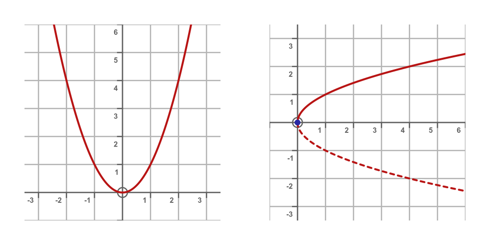
Over time, mathematicians developed the ideas of functions, inverse functions, and plotting functions as graphs. It is quite easy to plot the square root function, based on the square function. We can plot the square function simply by calculating x² for many different values of x, and then joining the points with a smooth line. To plot the square root function, we simply need to plot the same values, but interchange x and y (which is equivalent to flipping the entire graph over the leading diagonal). Here are graphs of x² (left) and root x (right):

We later gained an understanding of indices, and we now know that taking the square root is equivalent to raising a number to the power 1/2. But initially, having a method to calculate the square root for a given x, and knowing how to plot its graph, made the function useful. If we look at trigonometry functions like sin and cos, or logarithms, or exponential functions, they follow a similar pattern. These functions are no more or less valid than the Lambert W function, they are just more familiar.

Before moving on, there are a couple more observations we can make about the square root function:

• The graph doesn't exist for x < 0. We can't find the square root of a negative number (at least, not amongst the real numbers).
• The square root function is not actually a function, because for some values of x, there are two answers (-2 and +2 are both square roots of 4, for example). We normally get around this by saying that the square root function always returns a non-negative value. But we need to remember that an equation involving squares will usually have two solutions. On the graph, we have indicated this by showing the negative branch of the square root function as a dashed line.

Understanding the Lambert W function

So let's get to know the Lambert W function a little better. We can start by plotting its graph. We know how to plot the graph of G(x), it is just a normal function of y against x. Since the Lambert W function is the inverse of G(x), we can plot it using the same technique that we used to plot the square root function above. G(x) and the Lambert W function are shown on the left and right graphs below:

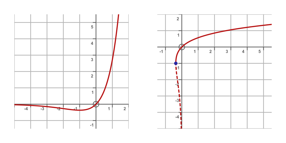
The blue point marked on the right-hand graph is the point (-1/e, -1). The Lambert W function is not defined to the left of this point, so, for example, we cannot find W(-1) in the same way that we cannot find the square root of -1.

Also, for some values of x, the Lambert W function has two possible values. In the square root case, we solved this by saying that the square root function always has a non-negative value. That works well because the curve is symmetrical about the x-axis.

For the Lambert W function, it is a bit more messy. For values of x that are greater than -1/e but less than 0, the function has two possible values, one of which is greater than -1, the other being less than -1.

We handle this by defining two branches of the Lambert W function. The first branch, called W₀ is defined for x ≥ -1/e and has W ≥ -1. This is shown as the solid line on the graph. The second branch, called W_-1 is defined for -1/e ≤ x < 0 and has W < -1. This is shown as the dashed line. This is similar to the situation with the square root of x. There may be two possible answers. We normally take the default (W₀) unless we happen to know that the alternative is required.

Finding the value W(x)

So we have our function W, how do we find the numerical value of W(x) for some value of x?

What would you do if you wanted to find the numerical value of the square root of some value x? Or the natural log? Or the cosine? You would probably use a calculator or a similar app. And that app would tell you the approximate value. In most cases, it can't tell you the exact value because it might well be an irrational number. A calculator can't tell you the exact numerical value of the square root of 2, because it has infinitely many, non-repeating digits.

The same is true of the Lambert W function. You won't find the Lambert W function on most ordinary calculator apps, but various maths websites, for example WolframAlpha, support it. Many programming languages have Lambert W functions. For example, if you are programming in Python, the scipy.special.lambertw function can be used.

How does the app calculate it? A common way, and we mentioned earlier, is the Newton-Raphson method. This starts with an initial value and uses an iterative formula that creates more and more accurate approximations until the required number of digits is obtained.

Application - x to the power x

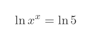
Now we will turn our attention to the original problem:

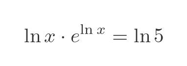
This bears a passing resemblance to our G(x) function, in that it is an expression involving x, and a power of x. Perhaps if we rearrange it, we might be able to absorb both x instances into G(x), and solve it using the Lambert W function. First, we can take the natural logarithm of both sides:

We will make use of the following basic logarithm identity:

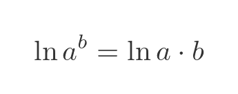
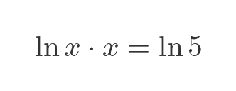
Applying this to the previous equation gives:

Next, we will apply the following identity. This works because ln x and e^x are inverse functions:

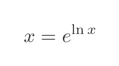
We use this to replace the factor of x in the previous equation:

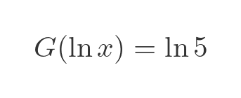
You might notice that the LHS of this equation looks like our earlier function G(x), but applied to ln x. Our definition of G(x) was:

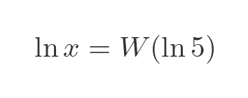
So we can write the previous equation as:

We know how to solve this. We can use the Lambert W function:

We can eliminate the log term on the LHS using the exponential function, so solve for x:

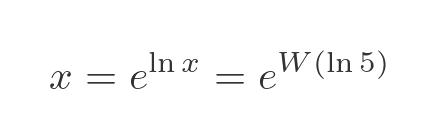
We can now solve this equation for x:

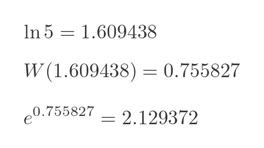
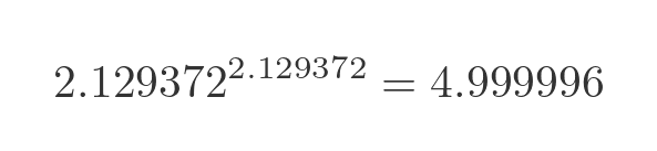
This looks plausible. 2 to the power 2 is 4, so you might expect slightly more than 2 raised to the power of slightly more than 2 to be equal to 5, and in fact it is:

See also

• The pi function