Pi isn't about circles

We usually associate π with circles. It is usually defined as the ratio of the circumference of a circle to its diameter.

This definition is quite correct, of course, and mathematicians have known about π for thousands of years. Mathematicians in ancient Babylonia, Egypt, Greece, India and China knew how to calculate π to a fair degree of accuracy. Archimedes calculated π to be about 3.14 using a geometric technique, around 200 BC. Chinese mathematician Zu Chongzhi calculated π to 7 digits around 500 CE.

It is not surprising that π is so strongly associated with circles as this is how mankind first came to know of it, and it is how most of us first learn about π at school.

But π has a far more fundamental definition, which is why it appears so often in more advanced mathematics that appears to have little to do with circles. In this article, we will see another side of π.

Trolley and spring

Suppose we have a heavy trolley, that runs on rails, attached to a fixed point by a spring. Here is the system at rest:

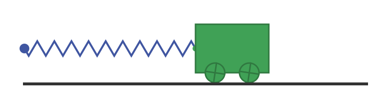
Let's say that the trolley weighs 1 kilogram, and the spring exerts 1 Newton of force for every metre it stretches. Let's also assume we can ignore friction, air resistance or any other effects.

A Newton is the standard unit of measure of force. One Newton is, fittingly, the approximate force that gravity exerts on an apple!

What happens if we pull the trolley along by 1m? Like this:

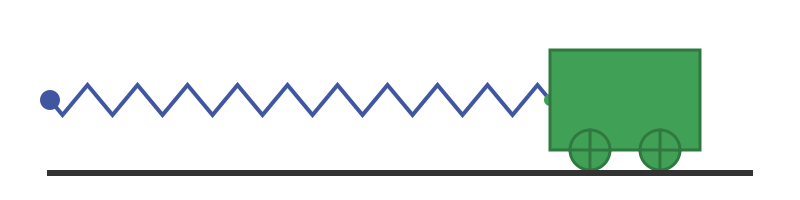
The spring is now in tension. It is pulling at the trolley with a force of 1 N, but we are resisting that force by holding the trolley in place.

If we let go of the trolley, the spring will pull it back towards the fixed point:

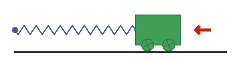
The force of the spring causes the trolley to accelerate. By the time the trolley reaches the mid-point, the spring is no longer in tension, so it is no longer pulling the trolley. However, the trolley now has gained momentum. It continues moving, which compresses the spring, slowing the trolley down. Eventually, the trolley stops, but now the spring is compressed which causes the trolley to start accelerating in the opposite direction. The motion is cyclic, as shown here:

If we assume a perfect system, the trolley will continue this motion forever.

How long does it take for the trolley to complete a cycle

All the important variables of the system have a value of 1. The trolley weight is 1 kg, the spring force is 1 N per metre of extension, and the spring is initially extended by a length of 1 m.

So how long does it take for the trolley to complete a cycle? You might guess it takes 1 second. Or maybe 1 second each way, so 2 seconds in total. Or something like that. You probably wouldn't guess that the time depends on some weird irrational number you learned about in school geometry lessons. Unless you read the title of this article, of course.

The equation of motion of the trolley

Now let's derive the equations that describe the motion of the trolley. This diagram shows the trolley:

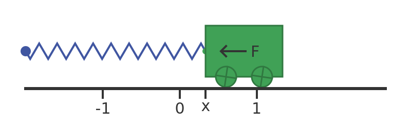
The rail is marked with points 0, which is the rest point of the trolley, and 1, which is the starting point before we release the trolley. The diagram shows the trolley at position x. It also shows the force F exerted by the spring.

The force exerted by a stretched spring is given by Hooke's Law:

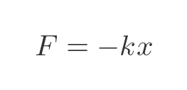
This means that the force F exerted by a spring is equal to the negative of extension x multiplied by the spring constant k. The negative sign is introduced because the force is always in the opposite direction to the extension. If we stretch the spring, the force tries to pull it back, and if we compress the spring the force tries to push back.

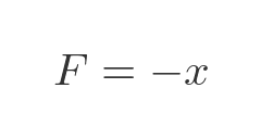
The spring constant, k, is a measure of how stiff the spring is, in other words, how much force it exerts if it is stretched (or compressed) by 1 m. We have previously said that, in this example, k = 1. So the force is:

How does the trolley move under the influence of this force? Well, a force accelerates an object according to Newton's second law - force equals mass times acceleration:

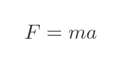
Again, we originally stated that the mass of the trolley is 1 kg so this equation simplifies:

We can express the acceleration in terms of x. We know that velocity is the rate of change of x, and acceleration is the rate of change of velocity. This means that acceleration is the rate of change of the rate of change of x. This can be written as the second derivative of x (in other words, x differentiated twice):

We now have two expressions for F, we can equate them to give an equation that describes the change of x over time:

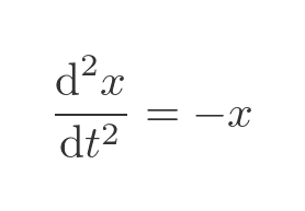
This type of equation is called a differential equation. If you are familiar with differential equations, you will understand what it means, and you might even recognise the standard solution. If not, don't worry. This equation tells us that x varies as a function of time t:

It also tells us that the function has a particular property - if we differentiate the function twice, the result is equal to the negative of the original function:

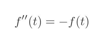
(The notation f' is shorthand for the derivative of f, f'' is shorthand for the second derivative of f, f''' is shorthand for the third derivative of f, etc)

That is almost enough information to tell us what the function is. Together with the initial conditions (for example, the position and velocity when t is 0) we can solve the equation.

Solving the equation

There are various ways to solve this equation. We will use the Maclaurin series to do it.

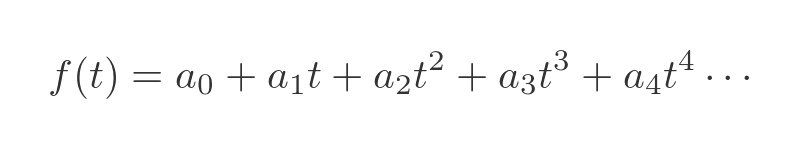
For this solution, we will assume that the equation takes the form of an infinite polynomial:

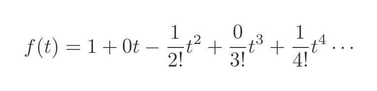
The Maclaurin method allows us to evaluate this expression numerically, to find an approximate solution. The solution is given by:

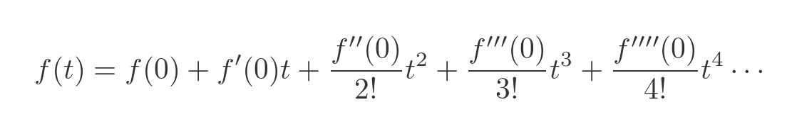
What does this mean? It tells us that the motion of the trolley is described as a polynomial function of time, where each term can be calculated in terms of the function f evaluated at 0.

Calculating a0

The first term, a0, is equal to f(0), that is the value of f when t is 0. But we don't know what the function f is, that is the whole point. So how can we calculate its value at 0?

Well, fortunately we don't need to know anything about the function f to calculate its value at time 0. f is equal to the position x. We know that the initial value of x (when t = 0) is 1 because that is where the trolley starts before we let it go. So a0 is 1.

Calculating a1

The second term, a1 is equal to f'(0). That is, the first derivative of f, evaluated at 0. But since we don't know what the function is, how can we differentiate it?

Once again, we don't need to know anything about f to calculate its derivative at t = 0. The first derivative of f represents the velocity of the trolley. And we know that at time 0 the trolley is stationary so the velocity is 0. So a1 is 0.

Calculating the other terms

It is clear that to solve the equation completely, we will need to find f''(0), f'''(0), and so on.

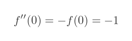
We can find f''(0) because the original differential equation was:

So it follows that:

We can find the third derivative, f'''(t), by differentiating the second derivative:

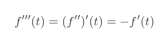
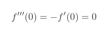
We have again used the fact that f''(t) is equal to -f(t). Evaluating this at 0 gives:

We can find the fouth derivative, f''''(t), by differentiating the second derivative twice:

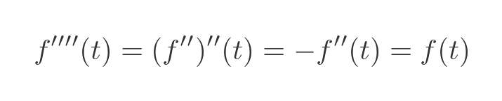
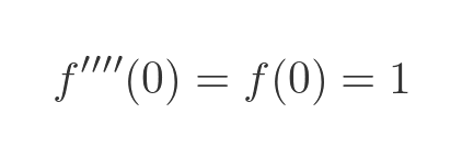
This time twice used the fact that f''(t) is equal to -f(t). Evaluating this at 0 gives:

The final formula for f(x)

The values of f(0), f'(0), f''(0) etc form a repeating cycle 1, 0, -1, 0, 1, 0, -1, 0...

We can plug these values into the Maclaurin formula to give:

Removing the 0 terms, and tidying up gives:

This is the formula that describes the motion of the trolley!

Plotting the motion of the trolley

How does the trolley actually behave? We can find out by plotting a graph of the equation above.

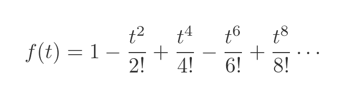
Here is the function calculated up to and including the term in t to the power 8:

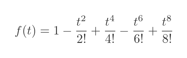
Notice this is a finite series, it contains no terms beyond t to the power 8. Here is a graph of this function:

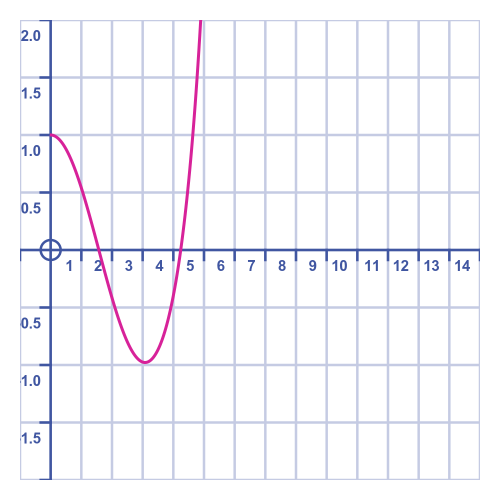
In this graph, the x-axis represents time, and the y-axis represents the position of the trolley.

The graph appears quite plausible at first. The trolley starts at x = 1, it speeds up as it approaches the midpoint x = 0, then slows down again as the spring compresses as it heads towards x = -1, where it slows to a halt then reverses its direction. If we were to do this experiment in real life we would see that it takes slightly more than 3 seconds to travel from +1 to -1, as the graph predicts.

However, the graph then zooms off to infinity. This is incorrect, of course. The problem is that we are only using 5 terms in our approximation, and when t gets bigger than about 4, the missing terms become important, so ignoring them gives a bad result.

Now let's try again with an extended formula, including terms right up to t to the 18th power:

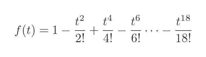
This is better:

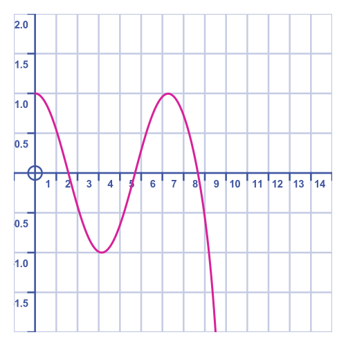
The graph shows the trolley going from 1 to -1 and back to 1, quite accurately. But about 8 seconds, things start to go haywire. This is for the same reason as before, that there aren't enough terms to model the function accurately for larger t values.

Finally, we will try using terms right up to t to the power 38:

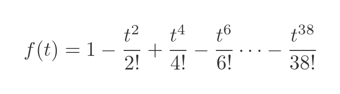
This shows, as we expected, that the trolley bounces backwards and forwards. In an ideal system with no friction or other losses, it will continue forever:

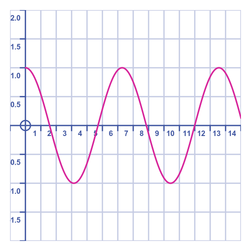
Even with all the extra terms in the equation, it will eventually go off course just like the other cases. But the motion is cyclic so if we can model the first cycle accurately we can simply repeat it for the other cycles.

How long does the trolley take to complete a cycle?

Back to our original question, how long does it take for the trolley to complete a cycle?

The trolley completes its first cycle when its position returns to 1. It is at the peak indicated by the red circle on this graph:

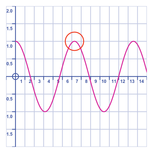
Visually we can see that this happens after 6-and-a-bit seconds. We can obtain a better approximation by calculating the formula above for several different values and funding the one closest to 1.

A process of trial and error tells us that the value is somewhere between 6.2830 and 6.2835. This table evaluates the function for various values between those 2 limits

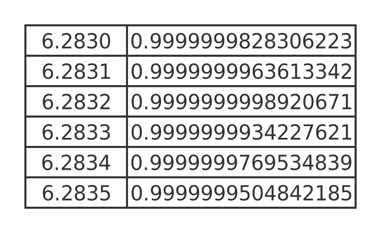
This tells us that the closest approximation to the trolley cycle time is 6.2832. That seems like quite a strange number, considering all the system parameters are equal to 1.

You might be aware that 2π is approximately 6.283185307. The value we obtained is very close to that.

If we repeat the experiment using a better approximation using more terms (for example using terms up to t to the power 100), we would find that the result is even closer to 2π. In fact, if we use enough terms in the equation, we can get as close to 2π as we like. Based on this, we can say that the exact periodicity is 2π.

You might also have noticed that this function looks suspiciously like the cosine function. That is because the Maclaurin series we have been using is the series for the cosine function. We won't prove it here, but the reason for this is that the second derivative of cosine is minus cosine:

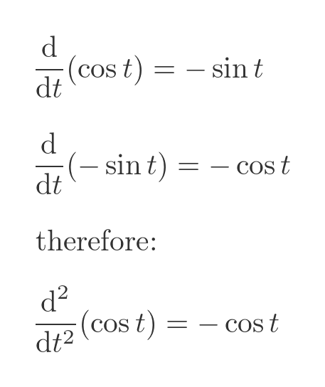
The cosine function, of course, has a periodicity of 2π, which further verifies the previous result.

So what is π?

π isn't about circles. It is actually related to the solution of a simple differential equation:

The solution to this equation is periodic, with a period that we will call τ (Greek letter tau). π is simply half of τ.

What about circles?

So why does π appear in the circle formula? Is it a coincidence? Well, no, when it comes to irrational numbers there is no such thing as a coincidence.

The circumference (arc length) and area of a circle are governed by the same differential equation as we use above, so the solution involves π. It is just that π was discovered in that context long before differential equations were known. But that is for a future article.

See also

• Calculating a Maclaurin series
• Maclaurin series of the exponential function
• Maclaurin series of the sine function