generativepy is an open source Python drawing library, mainly intended for maths/science illustrations and animations. It can be found on github.

The generativepy color module provides many features for handling color in diagrams. It includes:

• Support for RGB, Monochrone, HSL, and CSS named colors.
• Support for transparency (alpha channel) in all color modes.
• Color properties - for example individual r, g, or b values.
• Color modifiers - for example creating a darker version of a color, or interpolating between two colors.
• Color schemes - a flexible way to define a set of colors.
• Color maps - mapping integer values onto a varying color (covered in a later article).

The module uses the Color object to represent colors. Color objects are immutable - once a color has been created, it cannot be changed. If you need a different color, you must create a new color object. This avoids problems with color objects being changed while they are in use elsewhere, and it is similar to how Python treats number and string objects.

This module provides many ways to create new colors based on existing colors, as we will see later.

Creating RGB colors

We create a color object using the Color class, like this:

from generativepy.color import Color

color1 = Color(0, 1, 0)  # Pure green

When Color is called with three arguments, it creates an RGB color. The first argument controls the red value, the second controls the blue value, and the third controls the green value. A value of 1.0 turns that color fully on, and a value of 0.0 turns that color fully off.

A value of less than 0 is treated as 0, and a value greater than 1 is treated as 1.

The example above creates a 100% green color because the green value is 1 and the red and blue values are 0.

Creating RGBA colors

We can also create transparent colors, sometimes called RGBA colors. Here, A represent the alpha value, or opacity value—an A value of 1 creates a fully opaque color. An A value of 0 creates a fully transparent color, which means an object painted in that color is invisible.

We create an RGBA color by supplying a fourth parameter to the Color function:

color2 = Color(1, 0, 1, 0.8)  # Magenta with 80% opacity

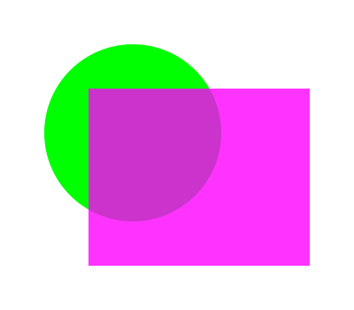
This creates a magenta color (red and blue both set to 1), but with an alpha value of 0.8. This means that the color is 80% opaque, so anything behind the object will be partly visible. This code is a circle with color1 behind a rectangle with color2:

from generativepy.color import Color
from generativepy.drawing import setup, make_image
from generativepy.geometry import Rectangle, Circle

def draw(ctx, width, height, fn, frame_count):
    setup(ctx, width, height, background=Color(1))

    Circle(ctx).of_center_radius((150, 150), 100).fill(color1)
    Rectangle(ctx).of_corner_size((100, 100), 250, 200).fill(color2)

make_image("alpha.png", draw, 400, 350)

Here is the image. Notice that the circle is still visible through the rectangle, even though the rectangle is drawn over part of the circle. That is because the rectangle is partly transparent:

The Color object

If we print the two color objects, we see something interesting:

print(color1) # prints rgba(0, 1, 0, 1)
print(color2) # prints rgba(1, 0, 1, 0.8)

A Color object always stores an RGBA value, even if the color is created with only RGB values. When we specify RGB values, the A value is automatically set to 1, which gives a fully opaque color.

Monochrome colors

If we call Color with one numerical parameter, it creates a monochrome color (ie a shade of grey). If we call it with two parameters, it creates a transparent shade of grey. Here is an example:

color3 = Color(0.7)
color4 = Color(0.4, 0.5)

print(color3) # prints rgba(0.7, 0.7, 0.7, 1)
print(color4) # prints rgba(0.4, 0.4, 0.4, 0.5)

def draw(ctx, width, height, fn, frame_count):
    setup(ctx, width, height, background=Color(1))

    Circle(ctx).of_center_radius((150, 150), 100).fill(color3)
    Rectangle(ctx).of_corner_size((100, 100), 250, 200).fill(color4)

make_image("grey.png", draw, 400, 350)

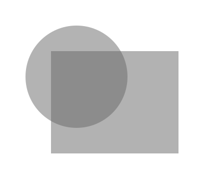
In this code, color3 is a grey color with grey value 0.7. When we print this color, we get rgba(0.7, 0.7, 0.7, 1). This is still an RGBA color, but with the red, green and blue values all set to 0.7, so it gives a grey color. The alpha value is set to 1 to create a fully opaque color, as in the RGB case. To create a transparent grey, we add a second parameter which serves as an A value. Here is the resulting image:

Named colors

We can also create CSS named colors. If the first parameter is a string that matches a CSS color name, then the corresponding color will be used. Once again, if there is a second parameter, it will be used to set the transparency:

color5 = Color("cadetblue")
color6 = Color("firebrick", 0.7)

def draw(ctx, width, height, fn, frame_count):
    setup(ctx, width, height, background=Color(1))

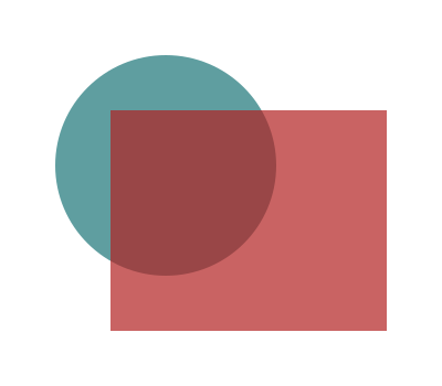
    Circle(ctx).of_center_radius((150, 150), 100).fill(color5)
    Rectangle(ctx).of_corner_size((100, 100), 250, 200).fill(color6)

make_image(FOLDER + "named.png", draw, 400, 350)

print(color5) # prints rgba(0.37254901960784315, 0.6196078431372549,
              #             0.6274509803921569, 1)
print(color6) # prints rgba(0.6980392156862745, 0.13333333333333333,
              #             0.13333333333333333, 0.7)

Here is the resulting image:

HSL colors

The hue, saturation, lightness (HSL) system is an alternative to RGB for specifying colors. It isn't actually a different color space; it is a remapping of the RGB color space onto HSL values. The three values in the HSL system are:

• Hue determines the basic color.
• Saturation determines how intense the color appears.
• Lightness determines how light the color appears.

HSL makes color more intuitive. If you have a particular color in mind, trying to find the correct RGB values to make that color can be very difficult. With HSL, you need to select the hue value that corresponds to the basic color you want. You can then vary the saturation and lightness to match exactly what you want. But the key thing is, changing the saturation and lightness doesn't affect the underlying color itself.

This diagram illustrates HSL:

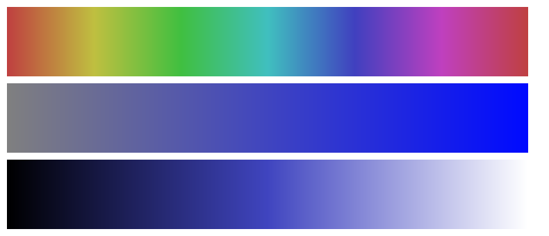
The top bar shows the hue, assuming a saturation of 0.5 and a lightness of 0.5. The hue starts at red (when H is 0), then it moves towards yellow (when H is about one sixth), then to green, cyan, blue, and magenta. Finally, as H goes towards 1, the color goes back to red. You can choose any base color using an H value between 0 and 1.

Let's imagine we picked an H value of two-thirds, which is blue. The second bar shows that same blue color with various saturation levels. If we move towards the right, the blue gets more saturated (you might say it is a purer blue, or a more intense blue). If we move to the left, the color gets less saturated, and starts to look more like a bluish grey. In fact, when the saturation is zero, the color will be pure grey. It doesn't matter what the hue is; when the saturation is zero, the color will be grey.

The bottom bar shows the lightness. Again, we are using the blue hue, and we will assume the saturation is 0.5. The lightness value controls how light the color is. Towards the left of the bar, where the lightness is low, the color gets darker and darker. When the lightness is 0, the color is black. Towards the right of the bar, where the lightness is high, the color gets lighter and lighter. When the lightness is 1, the color is white.

Every possible RGB color can be represented using HSL values, and every possible HSL color can be represented using RGB values. They are just different mappings of the same values. However, HSL values are often more intuitive.

Color properties

It is sometimes useful to find the individual RGB or HSL values of a color. We can do it like this:

color = Color("goldenrod")
red = color.r              # The red value
green = color.g            # The green value
blue = color.b             # The blue value
alpha = color.a            # The alpha value
hue = color.h              # The hue value
sat = color.s              # The saturation value
light = color.l            # The lightness value
rgb = color.rgb            # The color as a tuple of three floats
rgba = color.rgba          # The color as a tuple of four floats

Notice that all of these properties are available for all colors. For example, if a color is defined using RGB values, you can still find its hue. The single color properties return a single float in the range 0.0 to 1.0.

The rgb property returns the RGB values as a tuple of three floats representing the RGB colors. The rgba property returns the RGB values as a tuple of four floats representing the RGBA colors.

If you need to get the colors as byte values, you can use the following functions:

color = Color("goldenrod")
rgb = color.as_rgb_bytes   # The color as a tuple of three 
                           # integers in range 0 to 255
rgba = color.as_rgba_bytes # The color as a tuple of four
                           # integers in range 0 to 255

The as_rgbstr function is similar to as_rgb_bytes, but it returns a string containing the integer RGB values in the form:

"rgb(255, 128, 0)"

It can be useful for debugging.

Color modifiers

There are several ways to create a new color based on an existing color. For example:

color1 = Color("indigo")
color2 = color1.with_r(0.7)
color3 = color1.with_s(0.2)
color4 = color1.with_a(0.8)

Here are the four colors the code creates:

The square on the left is the original indigo color.

The next square shows the original color, but with the red component set to 0.7. This gives a slightly redder version of the color.

The next square shows the original color, but with the saturation set to 0.2. This gives a less saturated, or "greyer" version of the color.

The final square shows the original color, but with the alpha set to 0.8. This makes the color slightly transparent. It appears lighter because the white background of the page shows through.

There are modifiers for r, g, b, a, h, s, and l components.

There are also multiplier functions, for example:

color1 = Color("indigo")
color5 = color1.with_r_factor(2)

In this example, the original red value will be multiplied by 2 to create the new color. The result will be clamped to a maximum value of 1.

Again, of course, there are modifiers for r, g, b, a, h, s, and l components.

Finally, there are light and dark properties that create lighter and darker versions of a color:

color1 = Color("indigo")
color6 = color1.light1

The properties light1, light2, and light3 create increasingly lighter versions of the original color. The properties dark1, dark2 and dark3 create increasingly darker versions. These are just for convenience. If you want more control over exactly how dark or light the color should be, use with_l_factor to change the lightness of the color.

Color interpolation

Interpolation creates a color that is partway between two other colors. It is used like this:

new_color = color1.lerp(color2, 0.2)

In this code, color1 and color2 are two existing colors. The lerp function creates a new color that is partway between the two original colors.

Since the interpolation factor is 0.2, the new color will be approximately 80% color1 plus 20% color2.

Here is an example:

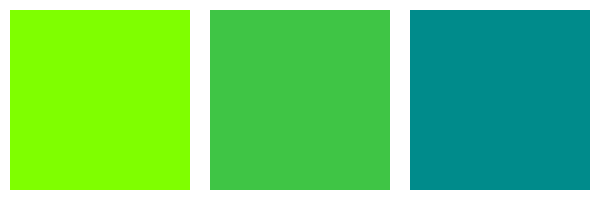
The square on the left is CSS Chartreuse, the square on the right is CSS Dark Cyan, the square in the middle is the color that is halfway between them.

Color schemes

Suppose you are creating images for a larger project. such as a website or book, it can be useful to use a standard set of colors across the whole project. Color schemes provide that.

A color scheme is a simple class that provides a set of colors as properties. You can define the set once and use it everywhere. The color module provides three color schemes:

• ArtisticColorScheme provides a general set of nice colors.
• DarkColorScheme provides a set of colors designed for a dark background. I use that for most of my YouTube videos.
• BookColorScheme is what I currently use for the newer articles on this website, as well as my printed books and ebooks. This color scheme provides regular colors RED, GREEN, etc. It also has lighter colors REDFILL, GREENFILL, etc, that can be used to fill shapes.

A color scheme is used like this:

from generativepy.color import Color, BookColorScheme

cs = BookColorScheme()

Line(ctx).of_start_end(a, b).stroke(cs.BLACK, 4)

But, of course, feel free to create your own color scheme, using the existing schemes as a template.

Related articles

• Introduction to generativepy
• Vector drawing with generativepy
• Graphs in generativepy