Drunk man and keys problem

The drunk man and keys problem is a simple but interesting probability problem.

A drunk man, returning home, is trying to open his house door with a bunch of keys. There are 10 keys in the bunch, but only 1 fits the door. He selects a key at random. If it fits the door he lets himself in, but if it doesn't fit he tries again. Because he is drunk, he doesn't remember which keys he has already tried, so he makes a totally random choice from the 10 keys each time.

The question is, on which attempt is he most likely to get in?

Some people think that the answer is 5 (because that is half of 10). Others say that there is no right answer because every time he tries he has exactly the same chance of picking the right key.

These might seem like reasonable answers, but they are answers to the wrong question.

In fact, he is most likely to get in on his first attempt!

A simulation

We will use some Python code that simulates the man trying to open the door. The code is very simple, so you should be able to follow the description even if you don't know Python.

We will number the keys from 1 to 10. The way we number the keys doesn't affect the outcome, so will assign number 1 to the correct key.

Here is the code. The function called simulation randomly tries key until it finds the correct one, and returns the number of attempts it took to get it right:

def simulation():
    tries = 1
    while True:
        guess = random.randint(1, 10)
        if guess == 1:
            return tries
        tries += 1

We first set the variable tries to 1.

Then we loop forever. Within the loop, we use randint to get a random integer in the range 1 to 10 inclusive, and store it in the variable guess.

Next, we check whether the random number is equal to 1, indicating that the correct key has been chosen. If it has, we exit the function and return the current value of tries.

If guess is not 1, we add 1 to the value of tries, and loop again. This means that the returned value in tries will be 1 if we find the key on the first try, 2 if we find it on the second try, and so on.

If we call this function 100,000 times and record the result each time, we get something like this:

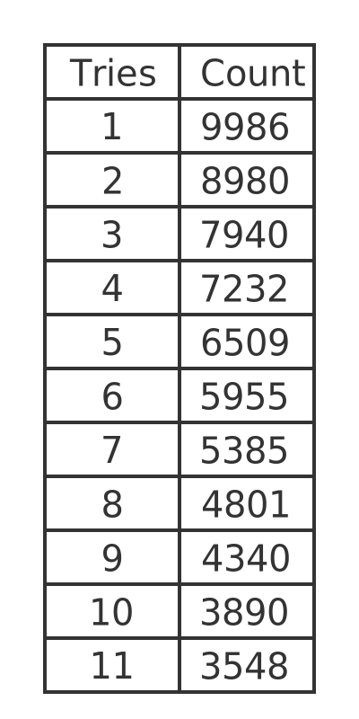
This means, for example, that 9986 times out of 100,000 tries the key was found on the first attempt. 8980 times it was found on the second attempt, etc.

Here are the same results expressed as a fraction of 100,000, rounded to 3 places. This gives the estimated probability of finding the key on the first attempt. second attempt, etc.

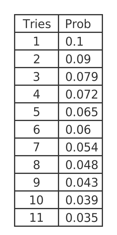
If you try this code yourself, you will most likely get slightly different results because it uses random numbers. But the differences will be small. One thing that will be clear, though, is that finding the correct key on the first attempt is more likely than any other attempt.

Why the wrong answers are wrong

If you answered 5, or similar, you might actually be answering a different question: what is the average number of attempts before the man opens the door? 5 is not a bad guess, although it isn't quite right (the actual number is greater than that). But it is answering the wrong question. More on this later.

If you answered that every time he tries he has exactly the same chance of picking the right key then you are, of course, quite correct, he always has a 1 in 10 chance of picking the right key.

But there is something else to consider. If he successfully opens the door on the first attempt, he will stop trying and go into the house. This consideration affects the probabilities.

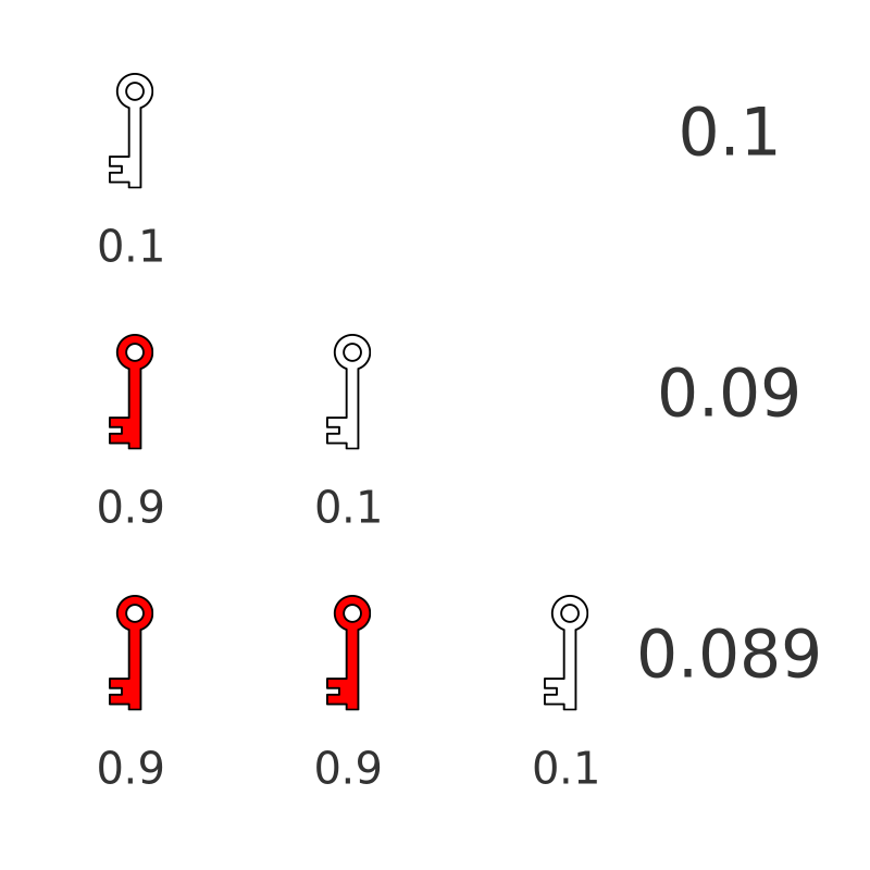
To open the door on his first try, he simply needs to find the right key on the first try, which has a probability of 0.1.

To open the door on the second try, 2 things need to happen. He must choose the wrong key on his first try. Then he must choose the correct key on his second try. The probability of getting the wrong key is 0.9, and the probability of getting the right key is 0.1. The probability of 2 independent events (choosing the wrong key, then choosing the right key) is found by multiplying the probabilities of the individual events.

So the probability of getting the right key on the second try is 0.9 × 0.1, which is 0.09. This is slightly less than the probability of getting it right the first time.

To open the door on the third try, 3 things need to happen. He must choose the wrong key on his first try, then again on the second try. Then he must choose the correct key on his third try. The probability of that is 0.9 × 0.9 × 0.1, or 0.081. This is slightly less than the probability of getting it right the second time.

Here is a diagram to illustrate this. It shows the probability of finding the right key on the first, second and third attempts:

The probability of getting it right on the nth attempt is:

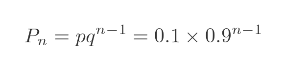
Here, p is the probability of success (0.1), and q is the probability of failure (1 - p or 0.9). Based on this formula we can create a table of the exact probability of finding the correct key on any particular attempt:

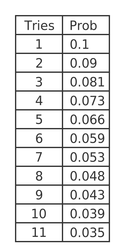
The table values are just the values from the previous formula, again rounded to 3 places. They match the random counts from our Python code remarkably well.

Average number of attempts

Now let's look at the other statistic we mentioned, which sometimes confuses people. What is the average number of attempts needed to find the correct key?

We know that the drunk man is more likely to find it on his first attempt than on any other attempt. But the chances are only 1 in 10, so he is very likely to need more than 1 attempt. How can we find the average number of attempts required to find the right key?

Finding the average from a running total

Here is the calculated table again, with a Totals column added:

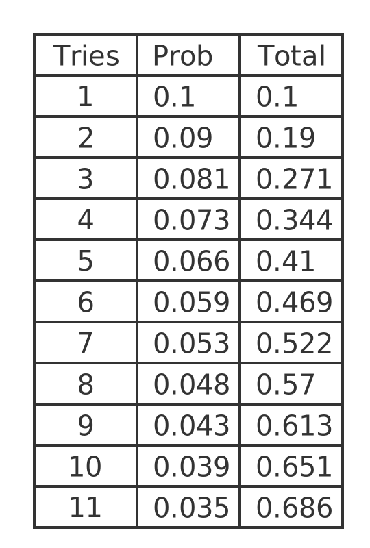
The new column is a running total of the values in the probability column. So for example, row 6 tells us that the probability of finding the correct key in 6 or fewer attempts is 0.469. The probability of finding the correct key in 7 or fewer attempts is 0.522.

So does this mean that, on average, it would take about 6.8 attempts to find the correct key? Well, not quite.

The table tells us the median number of attempts required. If we repeated this experiment lots of times, then in about half the experiments we would find the key 6 or fewer attempts, and the other half would take more than 7 or more attempts.

We are probably more interested in the mean number of times. This is likely to be somewhat higher. The times when we take 8 or 9 attempts to find the key contribute more to the mean than the times we take 2 or 3 attempts, which pushes up the mean.

Finding the average using the expectation value

The correct way to find the mean is to use the expectation value. This is given by:

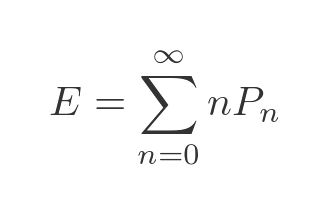
In other words, the average expected value is equal to the sum of every possible value multiplied by the probability of that value. Using the probability formula from before gives:

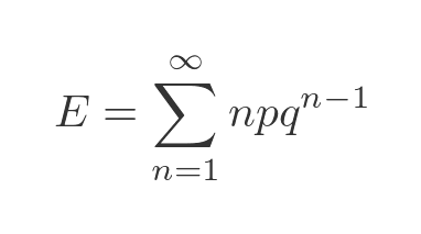
It turns out that this infinite sum evaluates to:

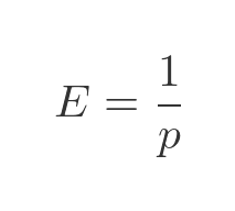
So in our case, with 10 keys, the average number of attempts before succeeding would be 10.

Proof

It isn't immediately obvious how to evaluate the infinite sum above, but the result can be proved quite easily.

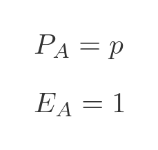
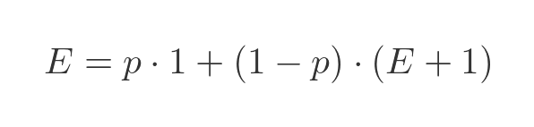
First, let's split the problem into two possible cases. Case A is that the key is found on the first attempt. The probability of that happening is p, and the expectation value is 1 (the correct key was found on the first attempt).

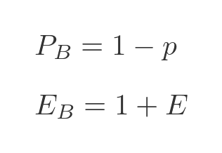
Case B is that the key is not found on the first attempt. The probability of that happening is 1 - p. What is the expectation value? Well in this case we intend to keep trying until we find the key, so the expectation value should be E, just like in the original case. But remember we have already tried and failed once, so we need to add 1 to take account i fthat extra attempt. The expectation value is therefore E + 1.

Since exactly one of the two cases A or B must occur, the overall expectation value is given by:

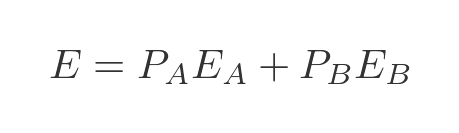
Substituting the previous values for the probabilities and expectation values gives:

This can be solved for E, giving the result:

This works in other cases too. For example. the average number of times you have to toss a coin to get heads is 2. The average number of times you have to roll a dice to get a 6 is 6.

See also

• Monty Hall problem
• Pigeonhole principle
• Raven paradox
• Painter's paradox
• Potato paradox
• Russell's paradox
• Coin rotation paradox