The Gaussian integral

This simple function has some important applications in mathematics:

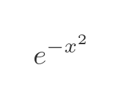
Since it is a function of x squared, it is an even function, and in fact creates the bell-shaped curve shown here:

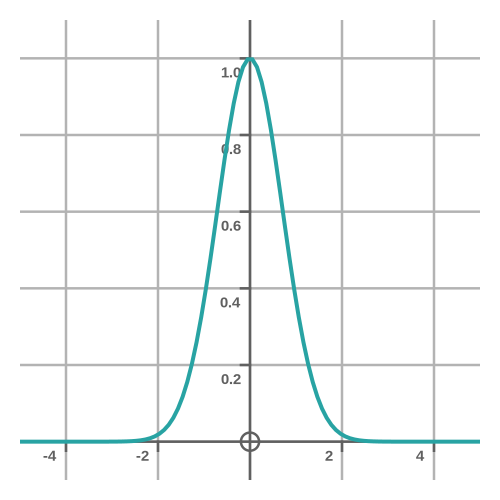
If this looks familiar, it's probably because it is closely related to the normal distribution in statistics.

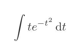
In this article, we will be looking at the following integral:

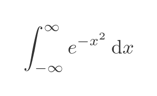
This is often called the Gaussian integral because Gauss was the first person to fully define it. It turns out that the indefinite integral has no elementary solution:

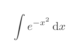
The error function, a special function, was developed to solve this integral. However, the definite integral above can be solved without requiring a special function. The solution does require quite a few steps, which we will work through in this article.

Overall approach

The general approach was originally suggested by Poisson, although there are now numerous versions. Looking at the integral, we can observe that it would be easy to solve if we could somehow get it into a form that resembles this:

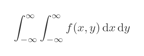
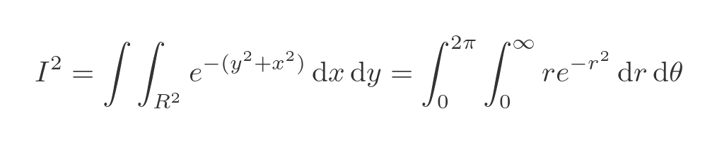
The extra t term would allow us to perform an integration by change of variable. But how do we get the integral into that form? There is a trick that can be used with double integrals:

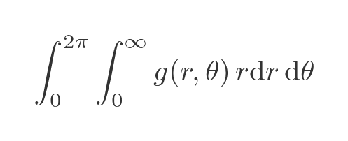
We can express this integral in polar coordinates. Here g is the equivalent function to f, but using polar coordinates:

Both integrals cover the entire XY plane because:

• In the first integral, x and y go from minus infinity to infinity.
• In the second integral, r goes from zero to infinity, and θ goes from 0 to 2π.

This means that the two integrals are equal. But notice that the polar form has an extra r term from the change of variables (for reasons we will see shortly). This looks quite promising! Let's look at this in more detail.

Converting the integral into a double integral

We will call our original integral I:

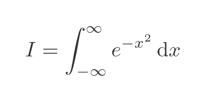
We can find I squared like this (we will see why this is useful, in a moment)

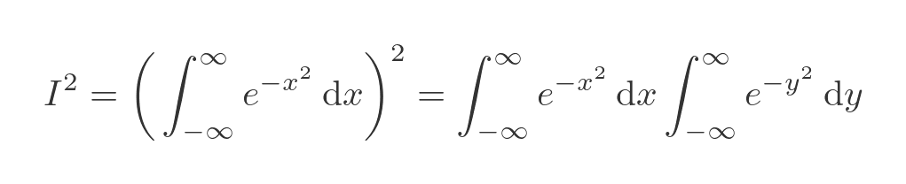
Notice in the second equation, we have used y instead of x. It is a definite integral, the name of the internal variable does not affect its value. In fact, we know that both integrals have the value I. If we substitute I for the x integral, we can do this:

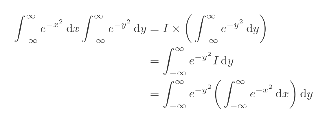
We have used the fact that the x integral is the constant I (it doesn't depend on y in any way) to allow us to move it inside the y integral. We then substitute the x integral for y again.

The second step is quite similar. The exponent in y squared doesn't depend on x in any way, it can be moved inside the x integral, giving:

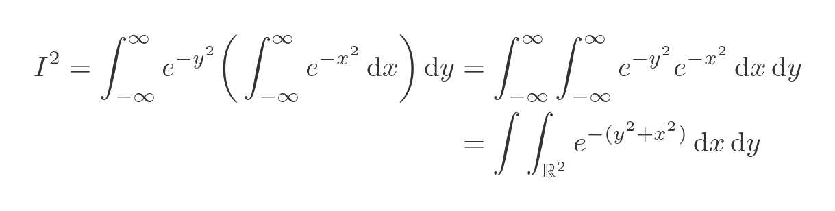
We have shown the double integral as being over ℝ² (the set of real numbers squared) to indicate that the integration takes place over the entire XY plane.

Looking at the function

So we are now looking at the function:

Here is a plot of the function, where the XY plane is the horizontal plane, and the value of the function is represented by the vertical axis:

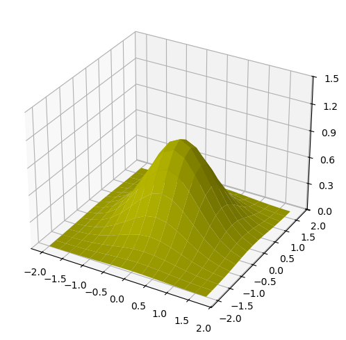
Our double integral, which we saw is equal to I², represents the volume under the curve.

Converting the integral to polar coordinates

Now we are ready to convert our double integral to polar coordinates. This is effectively a change of variables from x, y to r, θ.

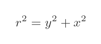
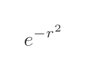
First, we need to express our function in terms of r, θ. This is, fortunately, quite easy. We know that, in polar coordinates:

So our integrand becomes:

This only depends on r, which will simplify things. We also need to convert from dx and dy to dr and dθ. The conversion is:

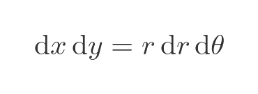
We will treat this as a known result that applies when we convert a double integral to polar coordinates. It is a bit beyond this article to prove it, but as justification, we can use this diagram:

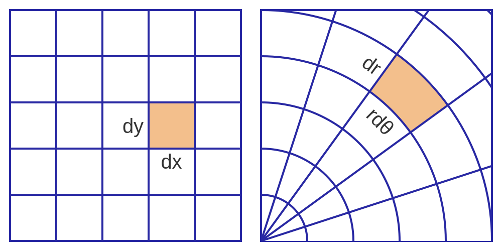
The volume under the function is found by multiplying the value of the function by the infinitesimal areas shown. In Cartesian coordinates, each infinitesimal area is an identical rectangle, with sides dx and dy. But in polar coordinates, the areas are not all the same, and have sides r dr and dθ. So we must substitute:

Here is the final integral, using the r and θ integration limits from earlier:

Evaluating the integral

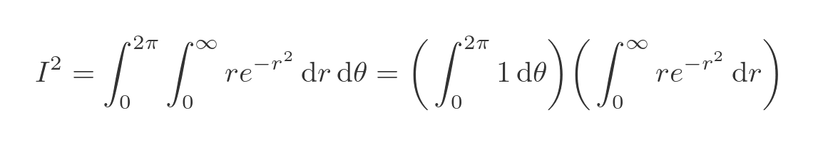
We still have a double integral, but the function only depends on r, and looks like a good candidate for a change of variables. But let's pretend the integrand is a product of two functions, a function of r and a function of θ. The function of θ just happens to be the constant value 1.

Earlier, we found the product of two integrals of functions in x and y, and combined them into a double integral of the product of the functions. Now we can do the same thing in reverse. We have a double integral of two functions in r and θ. So we can separate them:

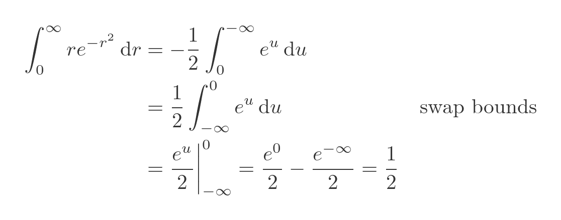
The integral in r can be solved by substitution, using:

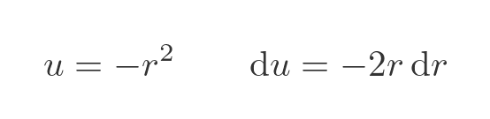
The negative sign here means we also need to change the bounds of the integral to the range zero to minus infinity. It is then a fairly straightforward integration by change of variable:

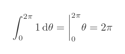
The integral of θ is much easier:

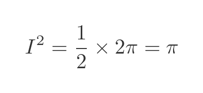
Multiplying these two results together gives us I²:

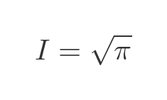
This gives us a final result for the Gaussian integral, which we have called I:

It is important to remember that this only works because we are integrating between negative and positive infinity. If we tried to integrate over a finite range, then our double integral would be over a finite square region. When we tried to convert the integral to polar coordinates, the bounds in polar coordinates would get messy. That is why the error function was created as a general solution to this integral.

See also

• The erf function
• The pi function
• The Lambert W function