The imaginary error function, erfi

The imaginary error function, erfi(x), is a close relative of the error function, erf(x). It is used for solving certain types of integrals, but it is also interesting in its own right.

The error function is described in detail here, but we will start with a brief description before moving on to erfi.

The error function

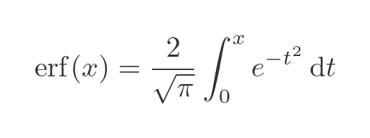
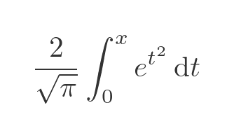
The error function is defined by the following equation:

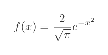
Notice that this is a function of x, not a function of t. That is because t is just the variable of integration. The value x determines the range over which the integral is calculated, which determines the final value of the integral. We will call the integrand f(x):

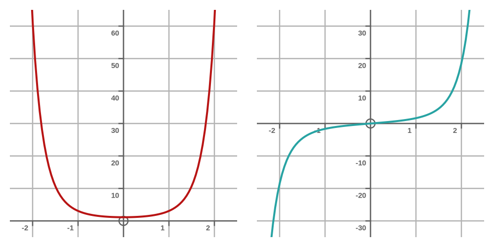
This graph shows f(x) on the left, and its integral erf(x) on the right:

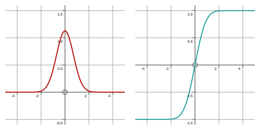
f(x) is a bell-shaped function. It is closely related to the normal distribution. The integral of the normal distribution is called the cumulative distribution function, and it is closely related to erf(x) (because erf(x) is the integral of f(x)).

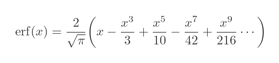
Now it turns out that the integral above is not an elementary integral. This means that it cannot be solved in terms of the usual functions such as sine, cosine, logarithms, etc. Instead, we define erf(x) as a special function. This means that we can solve the integral in terms of erf. For this solution to be useful, we need to be able to find the value of erf(x) for any given x (just like we can find the value of sin(x)). We can't always find the exact value of a special function, but we can find the approximate value to as many decimal places as we want. One way to do this for the erf function is the following Maclaurin expansion of the integral (which is proved in the linked article):

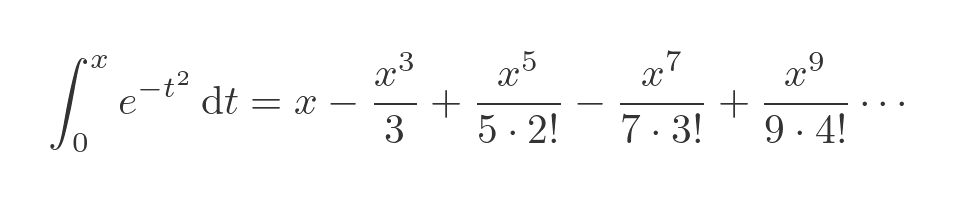
Adding in the multiplication factor and simplifying gives:

The erfi function

The erf function is very useful for working with probability distributions. But it might also be useful if we could solve integrals where the exponent is positive, such as this:

Here is a graph of the function on the left, and its integral (that we will calculate here) on the right. This time, the function is a U-shape rather than a bell. The function and its integral both get very big, very quickly, even for quite small values of x:

We could define another special function for this, but since this looks very similar to the integral used for the erf function, maybe we could use a variant of erf to solve it? So how can we change the -t² into +t²? Well, we know that if we square an imaginary number, we get a negative. So what if we find erf(ix) rather than erf(x)? This means changing the limit of the integral to ix:

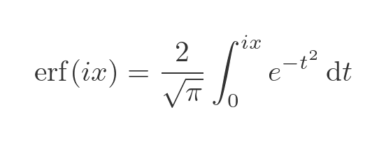
This might not seem to be much help. We now have a definite integral with an imaginary range, which is awkward. And it still has a negative exponent. Fortunately, there is a simple change in variables that will solve both problems at once. We will substitute:

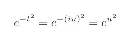
Remember that when we do an integration by substitution, we need to do three things. We need to substitute the variable in the integrand. When we do this, we get the square of iu, which cancels the negative in the exponent:

We also need to change the differential, dt. Since t is equal to u multiplied by i, and i is a constant, we need to apply the same factor to the differential:

Finally, since this is a definite integral, we need to change the limits of the integral to use u instead of t. The lower limit of 0 is unchanged (when t is zero, u is zero). For the upper limit, when t is ix, u is simply x (because we know that t = iu):

Making these three changes, we get:

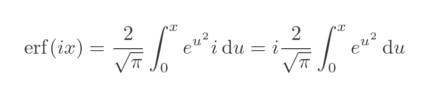
This is exactly what we need, except for that troublesome factor of i in the integral. We were able to take i outside the integral (again because it is a constant), but it would be nice to get rid of it altogether. We can do this by multiplying sides by -i, because, of course, -i times i is 1:

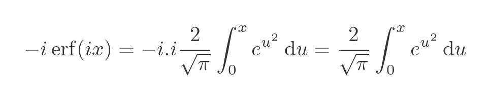
So we have our answer. But it is a very strange expression. What exactly are we supposed to do with it?

Calculating the integral

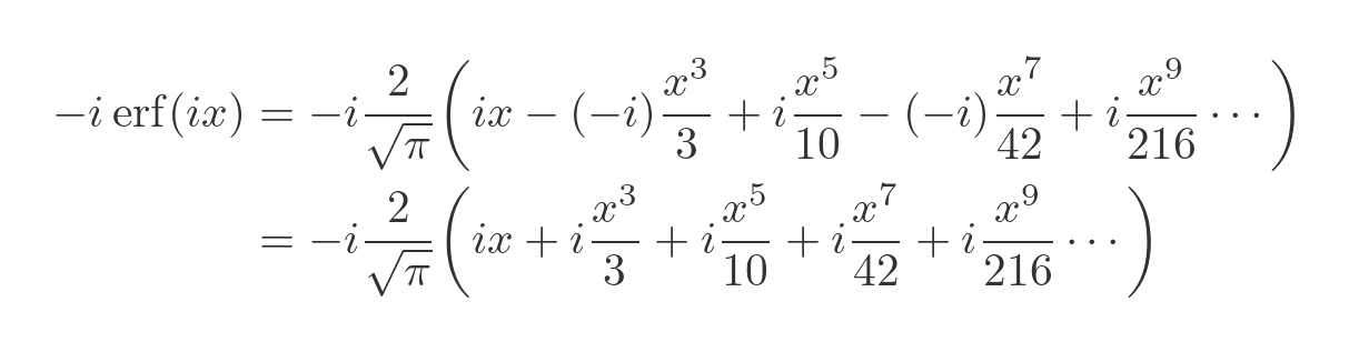
The result looks very odd, but let's trust the maths the brought us here. Remember that we know the Maclaurin expansion of the erf function. So we can use the Maclaurin expansion to find the erf function for any value, even if that value is imaginary:

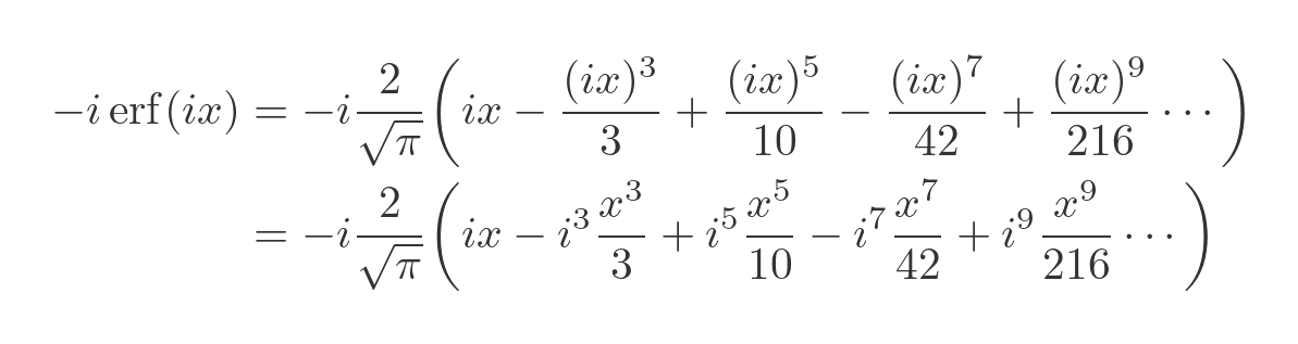
All we have done here is plug the value ix into the Maclaurin expansion, and multiply the whole thing by -i. The new expression contains odd factors of i. These terms simplify to alternating values of +/-i:

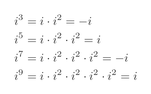
Applying this to the Maclaurin expansion gives us:

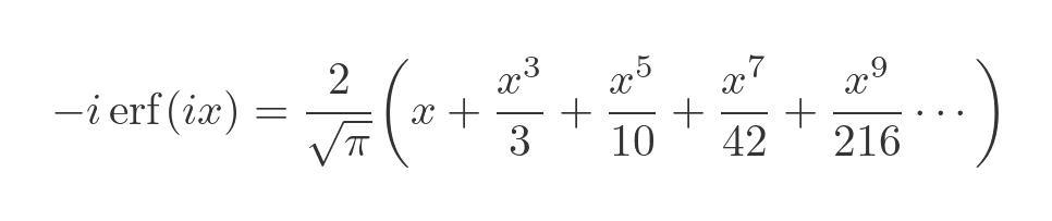
Notice that every term inside the brackets has a factor of i. We still have the factor of -i outside the brackets, and of course, the product of those terms is 1, so we can cancel all the i terms on the RHS:

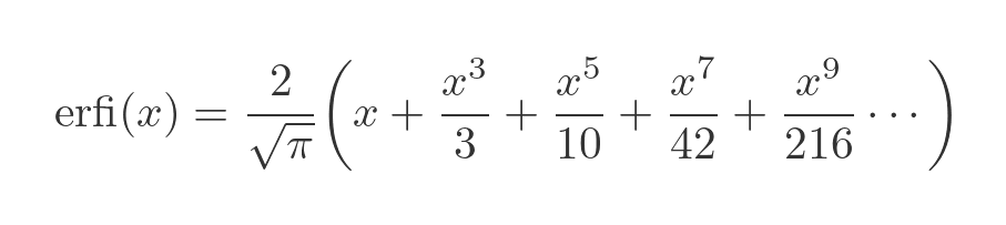
So the weird imaginary expression on the left has a real value. If we give it a name, the imaginary error function, or erfi, we can treat it as an ordinary function whose value can be calculated using the Maclaurin expansion (or other methods):

What just happened?

The result above might seem strange, perhaps even suspect. That is because, like the parable of the blind men and the elephant, we are looking at two aspects of the erf function but ignoring the whole thing.

In fact, the erf function is a complex-valued function of a complex variable. If we calculate erf(z) for any complex number z, we will get a complex number result w. Sometimes w will be purely real, sometimes it will be purely imaginary, but in most cases it will be a complex number with non-zero real and imaginary parts.

This diagram shows the complete erf function:

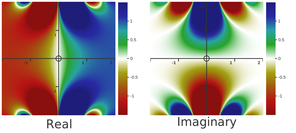
Each square area is an Argand diagram representing the complex input value z. The horizontal represents the real part of z, from -2 to +2. The vertical represents the imaginary part of z, from -2i to +2i.

The colours represent the value of the complex erf function. The left square is the real part of the erf function, the right square is the imaginary value.

The real erf function, that is erf(x) for real x, is just one small part of the complete function. It is the part of the function along the real axis, that is, the line where the imaginary part of z is zero. This is highlighted here:

Notice that, along the real axis, the imaginary part of the complex erf function is zero (shown as white). In other words, for real z, erf is a real-valued function. This is the real erf(x) function we used earlier.

The erfi function is found by looking at the imaginary axis:

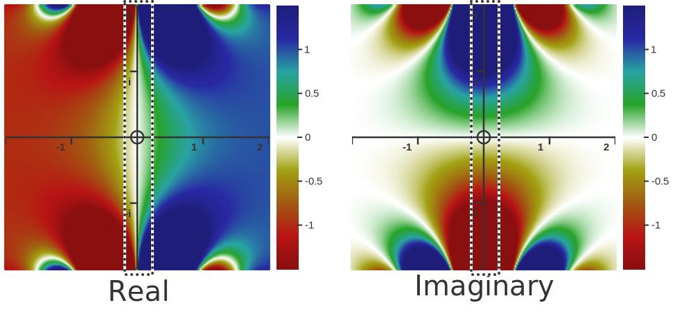
Along the imaginary axis, the real part of the complex erf function is zero. This means that, for imaginary z, erf is an imaginary function. This is the function erf(ix) we used earlier, which also yielded an imaginary result. If we multiply this function by -i, we get the real-valued erfi function.

Using the erfi function

The erfi function is available in many programming languages, although you might need to include a more specialised library. For example, in Python you can find the erfi function in the scipy library (scipy.special.erfi). This library also includes the complex-valued erf function (used to make the complex plots above). The regular, real-valued erf function is included in the standard math library for Python.

See also

• The Gaussian integral
• The erf function
• The pi function
• The gamma function
• The Lambert W function