Using Laplace transforms to solve simple differential equations

One important use of Laplace transforms is to solve differential equations. A differential equation is an equation that involves some function f(t) and its first derivative f'(t), second derivative f''(t), and possibly even higher order derivatives.

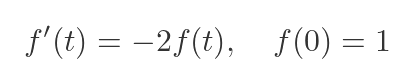
In particular, they are very useful for solving differential equations where the initial values are known. These are known as initial value problems or IVPs. A first-order IVP might look something like this:

There are various ways to solve simple equations like this. We will demonstrate the technique using Laplace transforms.

We will be using various Laplace transforms and inverse Laplace transforms. They can be found in any table of Laplace transforms, there are many available online.

How Laplace transforms help

Solving an IVP using Laplace transforms involves three steps:

• We apply the Laplace transform to the original IVP. This transforms the equation in t into an equivalent equation in s. In particular, the function f(t) is transformed into F(s).
• We solve the equation for F(s) as an expression involving only s.
• We then use the inverse Laplace transform to transform F(s) into f(t).

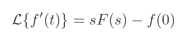
This will become clearer when we look at some examples, but first, it is useful to understand how this works. The original equation in t typically contains terms in f(t), f'(t), f''(t), and maybe higher derivatives. The Laplace transforms of these derivatives are standard, well-known results:

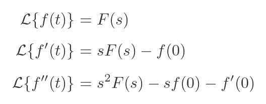
In these equations, f(0) and f'(0) are, of course, the values of f and its derivative when t is 0. In an IVP, these values will usually be given. In effect, they are constants.

The Laplace transform typically converts differential equations into purely algebraic equations that only involve F(s) and s. These equations can be solved for F(s) using simple algebra. Then F(s) can be converted back into f(t) using inverse Laplace transforms.

For very simple equations, there are other methods of solving IVPs that might be slightly easier. But we will use Laplace transforms to show how they work.

For more complex equations, and in particular for piecewise equations that contain step changes at various points in time, Laplace transforms can make things far easier.

Solving a simple first-order differential equation

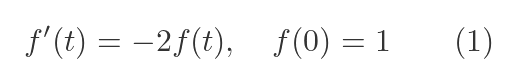
Let's see how to solve the previous equation:

We start by finding the Laplace transform of both sides. On the LHS, we need the Laplace transform of f'(t), which we saw earlier:

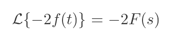
On the RHS, the Laplace transform of f(t) is, by definition, F(s). So we can find the transform of -2f(t) quite easily:

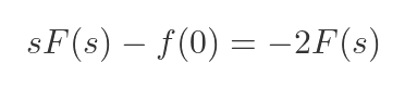
Substituting these two results into equation (1) gives:

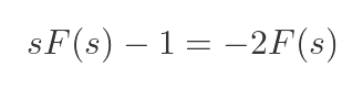
We have been told that f(0) is 1, so:

As described earlier, we can solve this equation by finding F(s) as a function of s. To do this, we gather all the terms in F(s) to the LHS, and simplify:

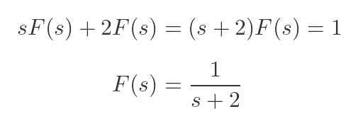
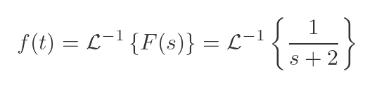
Since F(s) is the Laplace transform of f(t), it follows that f(t) is the inverse Laplace transform of F(s). So we can solve the IVP by taking the inverse Laplace transform of both sides:

The RHS looks very similar to this standard inverse transform:

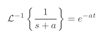
So we jut need to set a = 2 to find the solution:

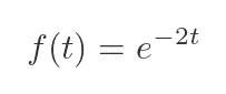
This answer looks quite plausible. The original equation is for a system where the rate of change of f is proportional to the negative of the value of f, and that is a classic example of a system exhibiting exponential decay.

Solving a simple second-order differential equation

This time, we will solve the following simple second-order IPV:

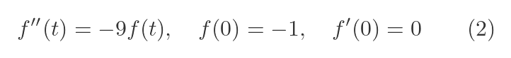
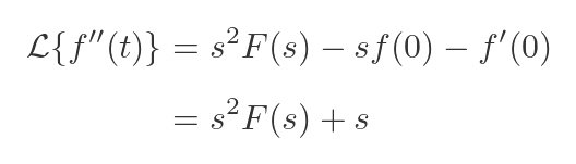
This time, the LHS is the second derivative of f. We know the Laplace transform of this from earlier. We can also simplify this by substituting the given values for f(0) and f'(0):

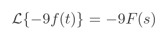
The LHS is similar to the previous equation:

Substituting this into equation (2) gives:

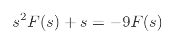
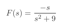
As before, we solve for F(s):

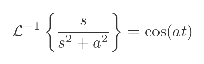
This expression is quite similar to the following inverse transform:

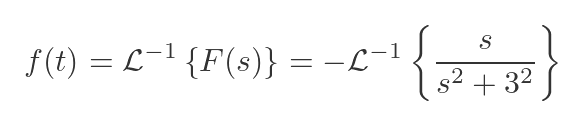
In this case, a squared is 9, so a is 3:

This gives the following result:

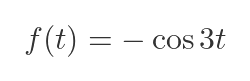
Once again, the answer looks plausible. The original equation is for a function whose second derivative is proportional to the square of its value, which indicates a sinusoidal function.

Related articles

• Introduction to Laplace transforms
• Laplace transforms of some simple functions