Complex sine and cosine functions

The sine and cosine functions are usually defined as real-valued functions, but it is possible to extend their definition to cover the complex domain. To do this, we make use of our previous definition of the complex exponential function.

This article will cover both functions, but will mainly concentrate on the cosine function, as it is slightly simpler.

Defining the complex sine and cosine functions

As we saw when looking at the complex exponential function, there is not necessarily any obvious right way to extend a function into the complex domain. We need to define how the complex function works, and then check that our definition makes sense - that it is consistent and useful.

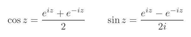
For the sine and cosine functions, our starting point might be Euler's equation:

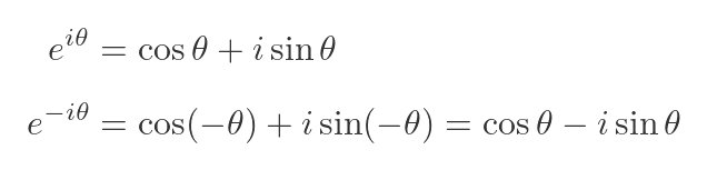
The second equation is just Euler's equation for -θ. Now, if we add these two equations, the two sin terms cancel out, so we get:

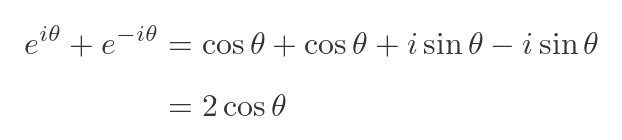
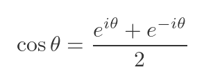
This gives us a nice expression for cos in terms of the imaginary exponential function:

As an aside, notice that we are still dealing with the real cosine function at this point. The expression on the right is a real-valued function of the real variable θ, even though the formula includes the imaginary unit i.

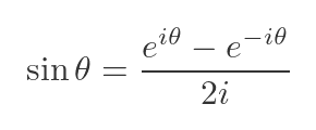
But a similar process, we can find the sine function (notice the i term in the denominator):

We might now define the complex sine and cosine functions, simply by replacing the real variable θ with a complex variable z:

And from the previous article on the complex exponential function, we know how to find the exponential of a complex number. So we can calculate the complex sine and cosine functions.

But that is based on our definition of what we mean by the complex sine and cosine. We still need to check that this definition is consistent and useful.

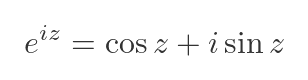
The complex form of Euler's equation

Using our new definitions of the sine and cosine of a complex number, we can now generalise Euler's equation to use a complex number z rather than a real value θ. The complex form is:

Here is the derivation:

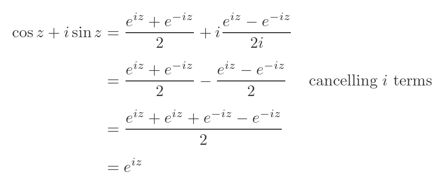
So that would seem to indicate that our definition of the complex sine and cosine is useful - it allows us to extend Euler's equation. Although that is not too surprising, since we assumed the extended form of Euler's equation in order to define the complex sine and cosine functions.

There is one important point to notice, though. In the original version of the formula, θ is real, so the sine and cosine values are real. So cos θ is the real part of the exponential, and i sin θ is the imaginary part.

In the complex version, z is complex, so cos z and i sin z are both complex numbers. The two terms longer represent the real and imaginary parts of the exponential.

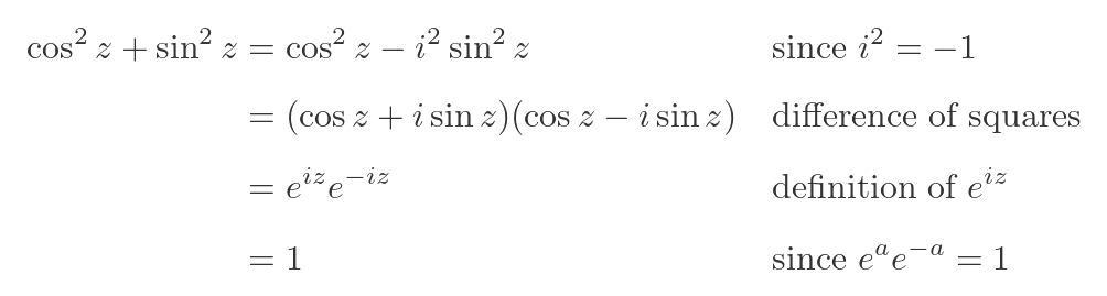
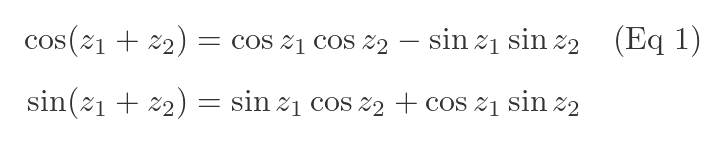
Complex trig identities

We can use the generalised version of Euler's equation to prove that many well-known trig identities still apply to the complex functions as we have defined them. We will just look at one example:

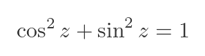
This can be shown using the complex version of Euler's formula:

Here are another couple of identities that we won't prove here, but will use later (they can be proved using similar techniques to the previous proof):

Taken together, the existence of these (and other) trig identities is one of the reasons we accept our definition of the complex trig functions as a valid and useful one.

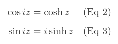
In the following sections, it will also be useful to know the following hyperbolic function identities, which again we won't prove here:

Real and imaginary parts of complex cosine

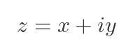
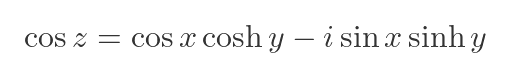
We will now take a more detailed look at the cosine function. We won't repeat this for the sine function, as the behaviour is quite similar. We have an expression for cos z, but it will be useful to express that in terms of the real and imaginary parts of z, which we will call x and y:

We can now find cos z using the various identities we introduced earlier:

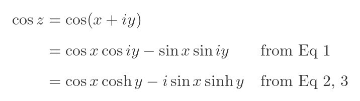
Now x and y are the real and imaginary parts of z, so they themselves are real values. So we now have an expression for cos z in terms of real functions.

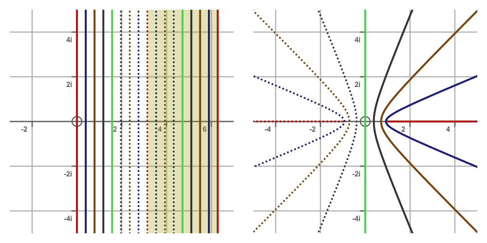
Mapping horizontal lines from z to w

We can start to get a handle on what this function looks like. We will first look at how horizontal lines (ie lines where the imaginary part of z is constant) map onto w (where w is cos z). Using the previous equation for cos z:

If we choose some value Y for the imaginary part of z (so that y = Y), this defines a horizontal line in the complex plane representing z. This line will map onto a set of values w that represents cos z for every z value on the line. The w values obey this formula, for every possible value of x (where x is the real part of z):

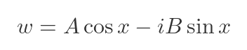
Where:

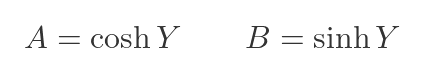
The formula for w represents an ellipse in the complex plane, with a width 2A in the real direction and a height 2B in the imaginary direction.

This is shown below. On the LHS, the various horizontal lines represent imaginary values (ie Y values) between -2 and +2. The RHS shows the corresponding curves in the w plane.

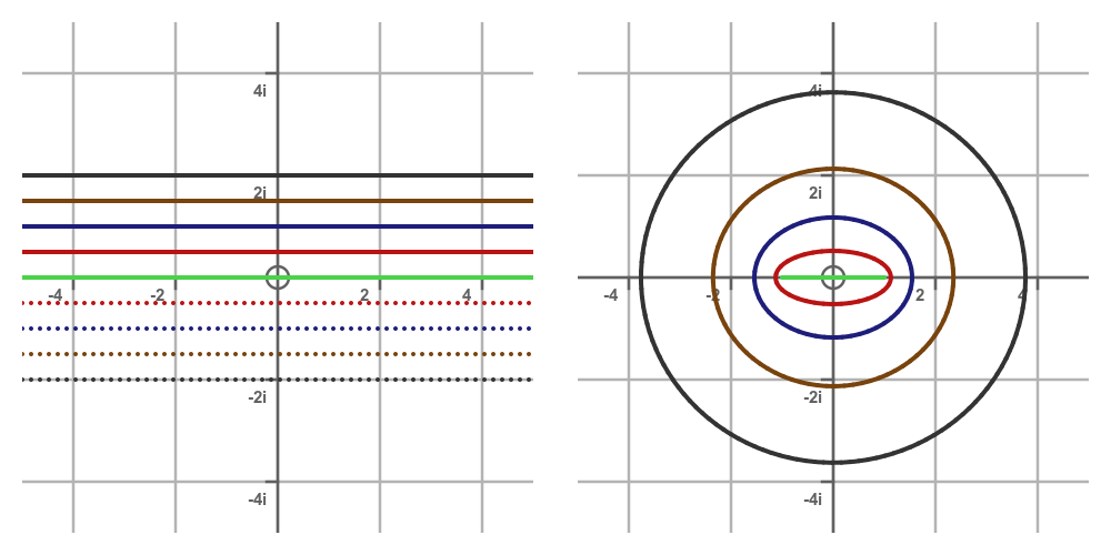
For example, the solid red line on the LHS has a Y value of 0.5. This means that A is about 1.13 and B is about 0.52, which gives the red ellipse on the RHS. There are some points to note:

• As Y gets bigger, A and B get bigger, so the ellipses get bigger.
• As Y gets bigger, cosh Y and sinh Y get closer together (see the sinh and cosh functions), so the ellipses become more and more circular.
• When Y is zero, A is 1 (because cosh 0 is 1) and B is 0 (because sinh 0 is 0), so the "ellipse" has zero height. That is, it becomes a line. It is shown as the light green line.

What about the dotted lines? They represent negative values of Y. The points fall on the same ellipse as the equivalent positive value, so they are not visible on the RHS. For example, the red dotted line maps onto the red ellipse.

Mapping vertical lines from z to w

For vertical lines in z, x has a constant value, which we will call X. So the sine and cosine terms of the expression for cos z are constant. This means that w obeys this formula:

Where:

This is a similar equation to the real case, but it uses the hyperbolic functions sine and cosine rather than the trig functions. This means that the equations define a hyperbola rather than a circle. This is shown here for various values of X:

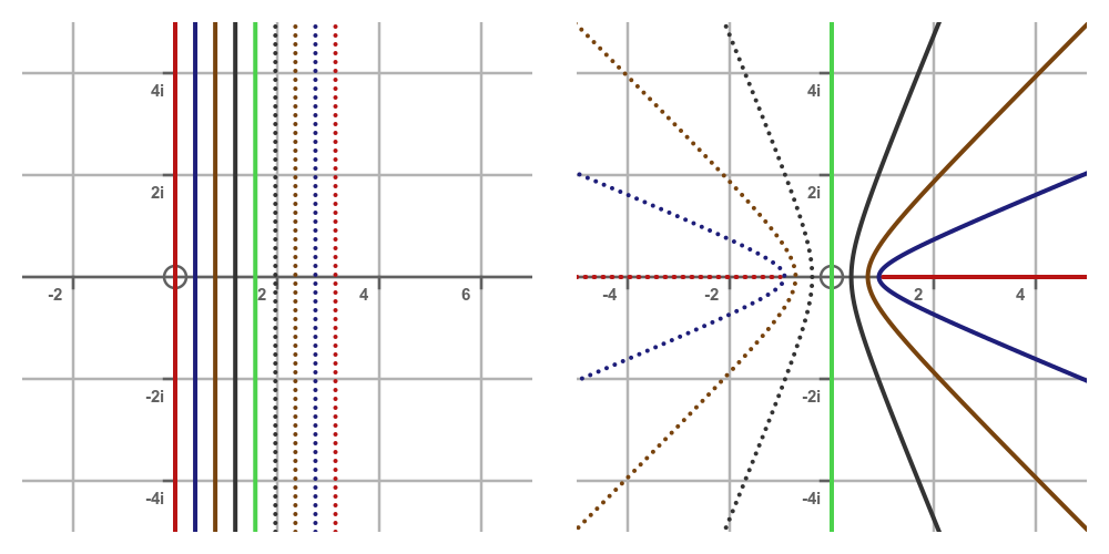
Here are some key points:

• The solid red line at X = 0 on the LHS corresponds to the solid red line along the y-axis on the RHS. This is a degenerate hyperbola that forms a straight line.
• The solid blue, gold and black lines correspond to the three hyperbolas.
• The solid green line, at X = π/2, creates another degenerate hyperbola, along the y-axis on the RHS.
• The dotted lines create additional hyperbolas with negative x-values on the RHS graph.

The complete set of hyperbolas produced by X values from 0 to π/2 completely fills the space on the RHS graph. But that isn't the whole story. Values of X from π/2 to π produce similar hyperbolas, but in progressing in the opposite direction (from the dotted red line to the solid red line, shown in the shaded area):

This pattern repeats along the real axis.

Mapping z to w

This diagram shows how various points in z map onto w. It combines the previous two graphs:

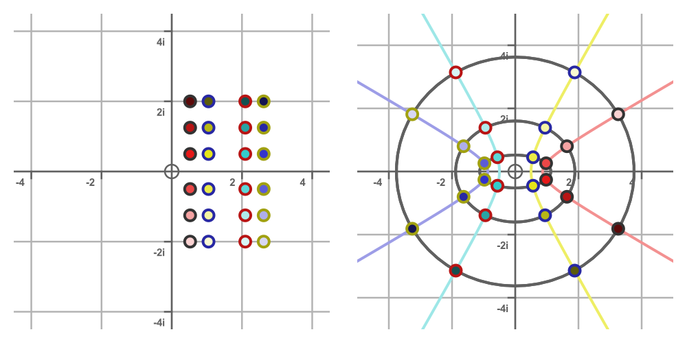
Notice that the 6 points with red centres (which have the same real value on the LHS z-value graph) all occupy the same hyperbola (with the light red line). Similar for the yellow, cyan and blue sets of points.

3D plots

Here is a 3D plot of the real part of the complex cosine function, with the equivalent heatmap on the RHS:

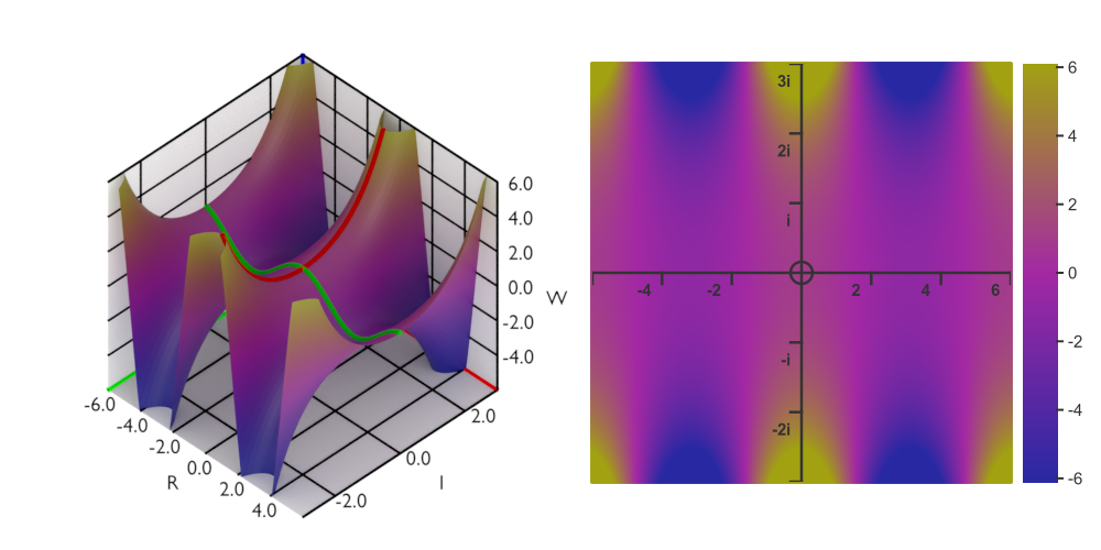
The green line on the graph represents the real part of w when Im(z) = 0. As we would expect, this is the cosine function. The red line represents the imaginary part of w when Re(z) = 0, which, of course, is the cosh function.

Here is the corresponding diagram for the imaginary part of the complex cosine:

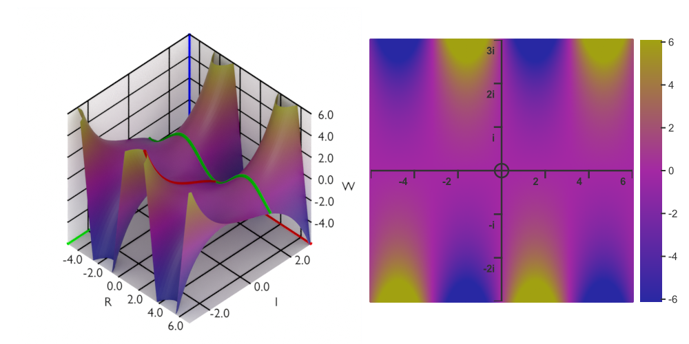
This time the green line represents the sine function, and the red line is the sinh function.

Related articles

• Complex exponential function
• Complex natural log function