Complex exponential function

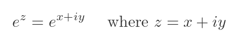
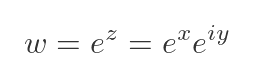
In this article, we will look at the complex exponential function, that is, the exponential function applied to a complex-valued argument z:

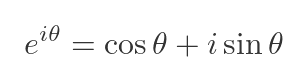
This function looks quite similar to Euler's formula:

There is a difference. Euler's formula has an imaginary exponent, whereas the complex exponential function has a complex exponent. But we will make use of Euler's formula to help us analyse the complex exponential function.

Defining the function

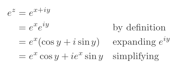
In the real domain, the exponential function of x is defined as e raised to the power x:

Here, e is Euler's number, a positive constant equal to approximately 2.7183.

We want to extend that function into the complex domain. It isn't obvious how we do that, because it involves raising e to a complex-valued power. We know how to raise a real number to a real power, for example, we know how to find x squared, or the cube root of x. But the meaning of a complex power is less obvious. We need to define what this means.

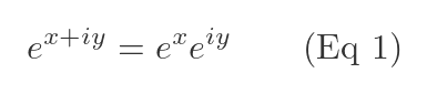
It turns out there is quite a simple way of doing this that is both intuitive and useful. We define the complex exponential function as:

This is analogous to the standard multiplication rule for real exponents a and b:

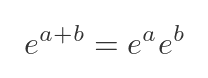
We are saying that, by definition, the rule applies to complex values as well as real values.

Why this definition is useful

Two things make this definition useful. The first is that we already know how to raise e to an imaginary power. Euler's formula tells us that:

So this definition allows us to calculate the actual value of the complex exponential:

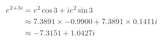
So, for example, e to the power 2 + 3i is:

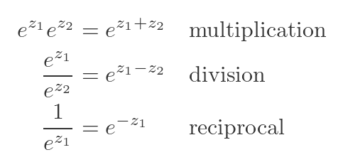
A second reason this definition is useful is that it means the normal rules for exponents also work for complex numbers:

Proof of multiplication rule for complex exponents

Before we delve further into this topic, we should probably prove the results above. After all, that is part of the justification for our definition. We will only prove the multiplication rule, the division and reciprocal rule proofs are very similar, so we won't show them here.

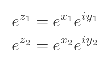
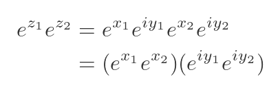
First, we can express the exponentials of the two complex numbers z₁ and z₂ in terms of their real and imaginary parts, using Eq 1 above:

So we can express the product of the exponentials like this:

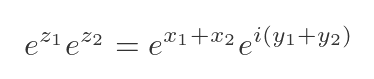
The first two exponentials have real exponents, x₁ and x₂. We know that the addition rule (above) applies in that case, it is just the ordinary real-valued exponential function.

What about the second two exponentials, which have imaginary exponents, iy₁ and iy₂? Well, you probably already know that the addition rule applies in that case too. When we multiply two complex numbers in polar form, we add the angles. We won't prove that here, we will take it as read. So we have:

Using those two results, we can write our complex product as:

Now this looks exactly like the RHS of Eq 1, it is the product of two exponentials, one with a real exponent, the other with an imaginary exponent. So we can use Eq 1 in the reverse direction to combine them:

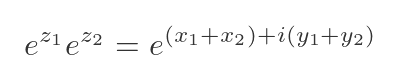
Now we have a single exponential, we can rearrange the terms in the exponent:

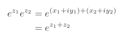
This proves the result.

A more useful expression of the function

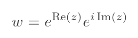
So far, we have come up with a definition of the exponential function and what it means to apply the exponential function to a complex value, and we have convinced ourselves that the definition looks quite useful. Now let's try to get a feel for how this function behaves. We will use w to represent the value of the function for some value z:

Since x is the real part of z and y is the imaginary part, we can replace them with the functions Re(z) and Im(z) that represent those real and imaginary parts:

This expression looks very similar to the (r, θ) form of a complex number, which expresses a complex number in terms of its modulus (as r) and its argument (as θ):

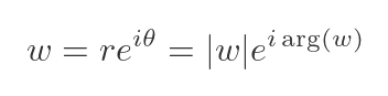
Comparing the terms in the two previous equations allows us to find the modulus and argument of w in terms of z:

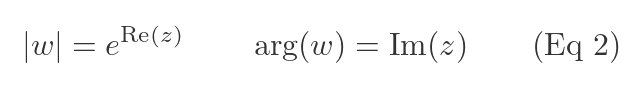
This is, in effect, a mapping of z values onto w values. For any number z, the mapping gives us a number w with the modulus and argument calculated by the equations above. Let's look at that mapping in more detail.

How horizontal lines are mapped from z to w

One way to get a handle on the mapping is to understand what happens when we transform horizontal and vertical lines from the z domain to the w domain.

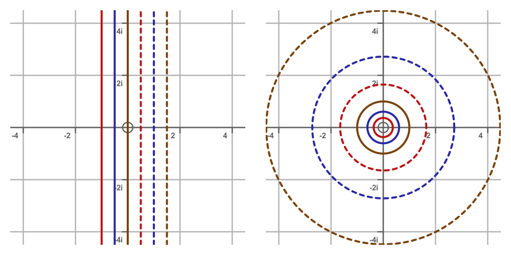
In the complex plane (represented on an Argand diagram), a horizontal line represents all the points that have the same imaginary part. For example, the line on the graph on the left below shows all the numbers z that have an imaginary part of π/3:

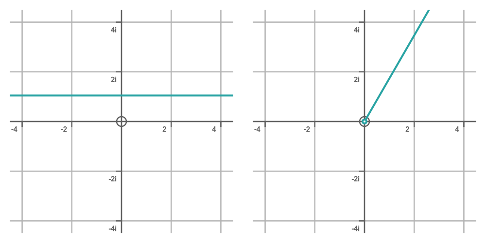
The line represents the set of numbers where Im(z) = π/3, for all possible values of Re(z).

What is the corresponding set of transformed numbers? Well, since Im(z) is fixed, we know that all the matching values of w must have an argument of π/3.

And since Re(z) can take any value, we know that matching values of w can have any positive modulus (because the exponential function in Eq 2 always has a positive value).

So matching values of w have arg(w) = π/3 for all positive values of |w|. This is the half-line from the origin at an angle of π/3 radians from the x-axis. This is shown in the RHS of the graph above. This does not include the origin, because |w| cannot be zero. That is indicated by the small circle at the origin.

This graph shows some other horizontal lines in z (left), with the corresponding half-line in w (right):

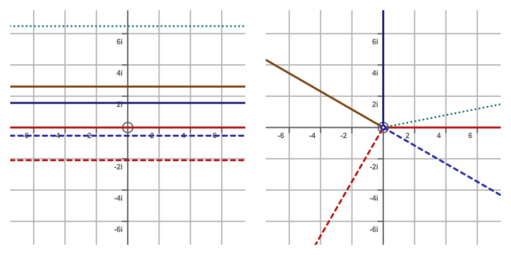
The lines are:

• Red solid, Im(z) = 0, corresponding to w values along the positive-going real axis (angle 0 rads).
• Blue solid, Im(z) = π/2, corresponding to w values along the positive-going imaginary axis (angle π/2 rads).
• Gold solid, Im(z) = 5π/6, corresponding to w values along the half line angle 5π/6 rads.
• Red dashed, Im(z) = -π/6, corresponding to w values along the half line angle π/6 rads clockwise.
• Blue dashed, Im(z) = -2π/3, corresponding to w values along the half line angle 2π/3 rads clockwise.

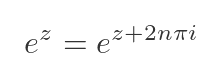
The cyan dotted line has an angle of 33π/16, or 2π + π/16. Since we are using the polar representation, this is equivalent to an argument of π/16. This means that the complex exponential is cyclical on the imaginary axis. That is to say, adding any integer multiple of 2πi to z does not affect the value of the exponential function:

How vertical lines are mapped from z to w

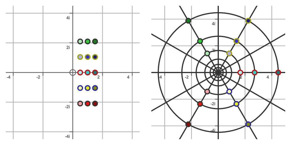
Now let's look at vertical lines. A vertical line represents all the points that have the same real part. For example, the line on the graph on the left below shows all the numbers z that have a real part of 1:

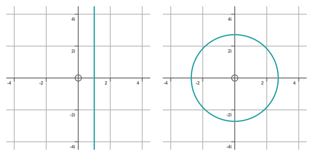
From the Eq 2, we know that the real part of z affects the modulus of w. In fact, the modulus of w is given by the exponential of the real part of z. So when Re(z) is 1 we have:

We also know that the imaginary part of z controls the arg(w). The vertical line represents all the values of z with a real part of 1 and all possible imaginary parts. In the w domain that maps onto all values of w that have a modulus of e and any possible angle.

That, of course, is a circle of radius e.

If we repeat this for different vertical lines, we would expect each line to map onto a circle with a different radius:

The solid gold line has Im(z) of 0, so it maps onto the unit circle in w (because e to the power 0 is 1).

The solid blue and red lines have increasing negative values of Im(z), so they map onto circles in w that have radii smaller than 1 (because e to a negative power is less than 1). The dashed red, blue and gold lines have increasingly positive Im(z) so they create circles with radii greater than 1.

Due to the exponential term, as the value of Im(z) increases linearly, the radii of the circles increase exponentially.

Interpreting the mapping as a change of coordinates

AS we have seen, the modulus of w depends only on Re(z), and the argument depends only on Im(z). So mapping from z to w is a bit like taking points in Cartesian coordinates and using them as if they were polar coordinates. Remembering the difference, of course, that the modulus is the exponential of the real part.

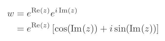
So any point in z can be mapped onto its equivalent point in w like this:

The LHS shows some different z values. The basic colour and outline of each dot indicates its imaginary part. For any given imaginary value, the basic colour is the same, but gets darker as the real value increases.

The RHS shows how these values are mapped onto equivalent w values:

• All points with the same imaginary part of z are on the same radial line (because they all have the same arg(w) value),
• All points with the same real part of z are on the same circle (because they all have the same |w| value).

The complete exponential function

We can gain a little more insight into this function if we expand the imaginary exponential term, using Euler's formula:

So the real and imaginary parts of w are given by:

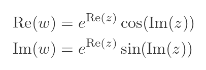
Looking at just the real part of w, it is equal to an exponential multiplied by a cosine. Here are the exponential and cosine terms on separate graphs:

The LHS shows the exponential function. As we travel along the positive-going real axis of z (the red line), we see that the value of the exponential function starts off very small (close to zero) but rapidly increases. This function does not depend on the imaginary part of z at all.

The RHS shows the cosine function. As we travel along the imaginary axis (the green line), the function oscillates between +1 and -1. This function does not depend on the real part of z.

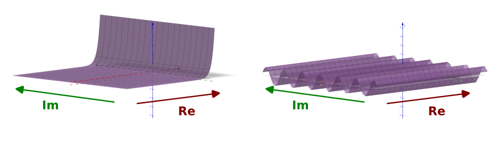
What happens when we multiply these two terms? The function oscillates along the imaginary axis, but the magnitude of the oscillation increases along the real axis.

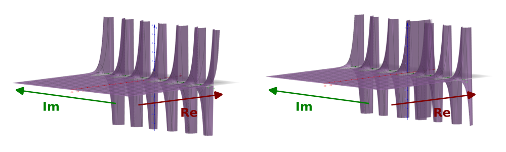
The LHS, above, shows the real part of w. The RHS shows the imaginary part. The two functions are very similar, but the oscillations in the imaginary direction follow the sine function rather than the cosine.

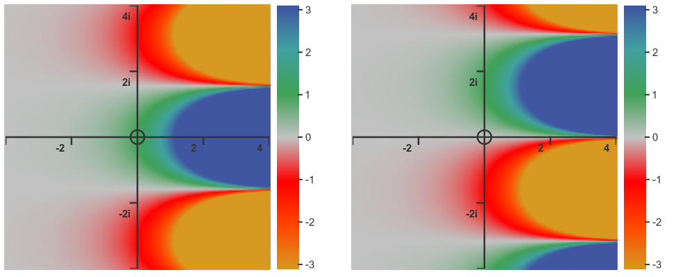
The graph below shows the same function as a heat map:

Summary

Like any complex function, the complex exponential function maps one set of complex numbers onto another. This involves 4 dimensions, so it can be difficult to visualise. It is often useful to look at a complex function from several different angles to fully understand it.