Area under a polar function

The familiar xy-plane uses Cartesian coordinates to represent points in a 2D space. Every point in space can be represented by a pair of (x, y) coordinates, representing the distance of the point from the origin in the x and y directions.

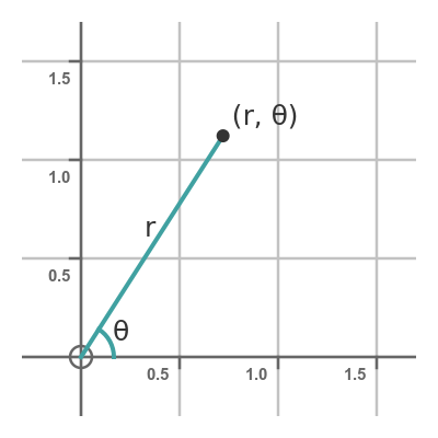
There is an alternative coordinate system, polar coordinates. In this system, the position of each point is represented by r (the straight line distance of the point from the origin) and θ (the angle the point makes with the x-axis at the origin). That is shown here:

It is possible to define functions using this coordinate system. For example, here is a spiral function:

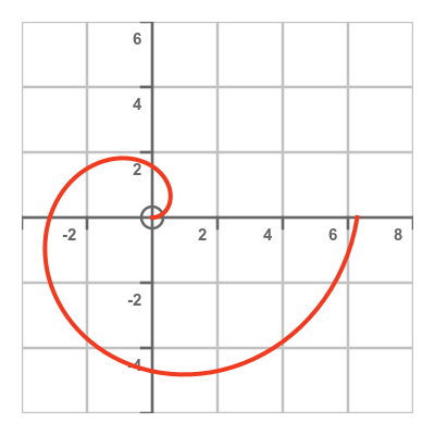
It is also possible to find the area under a polar function, and that is what we will cover in this article.

We will look at how to calculate the area under a polar curve using three simple examples - a circle, and spiral, and a cardioid shape. We will also see how to calculate the area enclosed between two curves.

Polar functions

In Cartesian coordinates, it is common to define an equation y = f(x). We can plot the function f(x) by drawing a curve through every point that satisfies the equation.

In polar coordinates, we can do a similar thing. We can define r = f(θ). We can plot the polar function f(θ) by allowing θ to vary and calculating the value of r for each value of θ. This animation shows how we can draw a shape this way:

Area under polar curve

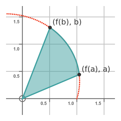
We can define the area under a polar curve, between two angles a and b. It is the area enclosed by the curve and the two straight lines from the origin to either end of the curve section, like this:

How can we calculate this area? As you might have guessed, we use integration to calculate this area. However, the calculation is slightly different to the method we use to find the area under a Cartesian curve.

Calculating the integral

To find the area under a curve in Cartesian coordinates, we often start by dividing the area under the curve into n small rectangles. The height of each rectangle is equal to the value of the function at the left-hand edge of the rectangle, as shown here:

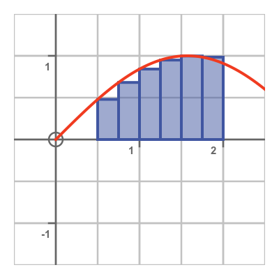
We find the sum of the areas of all the rectangles. This gives an approximation to the area under the curve. If we then double the number of rectangles, while making each rectangle half the width, we will usually end up with a better approximation to the area.

We repeat this process over and over, and each time the number of rectangles doubles, the width of each rectangle halves, and the approximation gets better. As the number of rectangles n tends to infinity (and the widths tend to zero) the sum becomes an integral giving the exact area under the curve.

We can do the same thing with the area under a polar curve r = f(θ), as shown here:

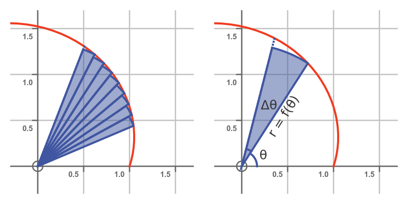
Again, we divide the area under the curve into lots of smaller areas. But instead of using rectangles, each smaller shape is a sector of a circle.

The RHS of the diagram shows one individual sector, made a little larger. We can see that the radius of the sector is equal to f(θ), and the angle of the sector is equal to a small angle that we will call Δθ.

We can calculate the area of the sector using the standard formula. If the sector has a radius R and an angle t (in radians) its area is given by:

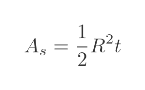
In our case, R is f(θ) and t is Δθ, so the area of the sector is:

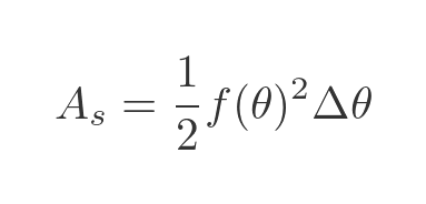
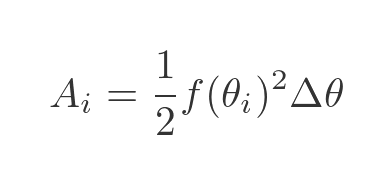
The total area under the curve (the LHS of the diagram above) is the sum of all the sector areas. There are n sectors, which we will number 1 to n. Sector i starts at θi, and all the sectors have an internal angle of Δθ. So the area of sector i is:

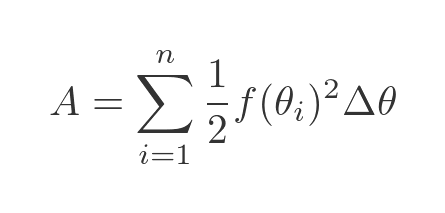
The total area is found by summing all these areas from 1 to n:

We won't prove it here, but as n tends to infinity and Δθ tends to zero, the sum becomes an integral:

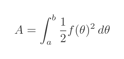
For any polar function f(θ) we can use this integral to calculate the area under the curve.

Example - a unit circle

As a simple example, and to test against a known result, we can use polar integration to find the area of a unit circle:

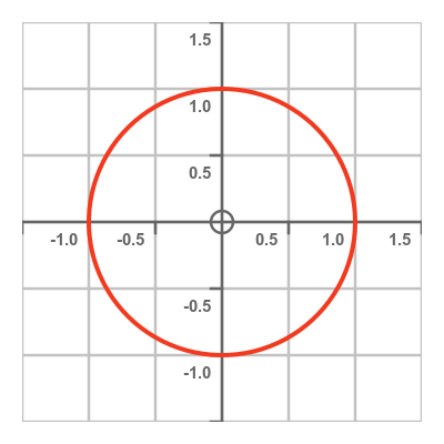
In polar coordinates, the unit circle has a very simple formula. For any value of θ, the distance from the origin to the curve is 1. So f(θ) has a constant value of 1 (it is independent of θ). The area integral is therefore:

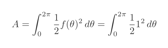
The integral of 1 from 0 to 2π is 2π, so:

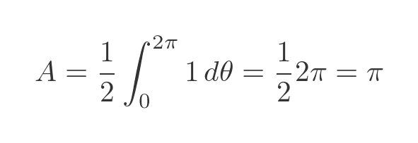
This gives the area of a unit circle as π. Of course, we already that from basic geometry.

Example - spiral function

The function r = θ is a spiral function:

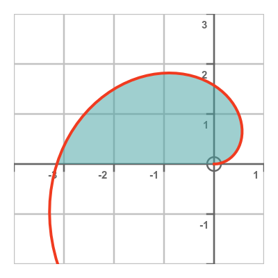
We will find the area under the curve between 0 and π (ie the area above the x-axis). If we substitute f(θ) = θ into the polar area equation we get:

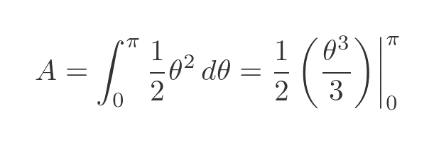
We have used the standard integral for θ squared. This evaluates to:

Looking at the graph, this result seems plausible. The shaded region looks like it is slightly more than 5 grid squares in area.

Example - cardioid curve

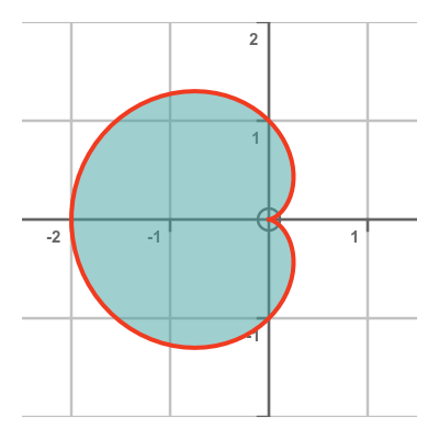
The cardioid curve has the following function:

Here is the curve it creates:

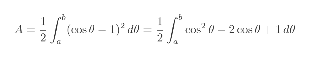
We find the area using the polar area integral from earlier:

We substitute our f(θ) and multiply out the squared term:

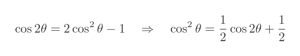
We will use the standard double-angle formula to simplify the cosine squared term:

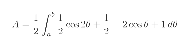
Substituting this back into the integral gives:

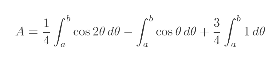
This simplifies to:

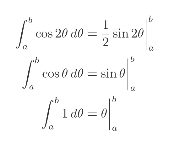
The first integral can be solved quite easily by substituting u = 2θ (the technique is covered here). The other two are standard integrals:

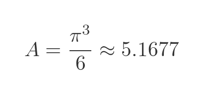
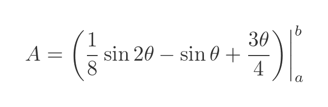
This gives a final result:

To find the area of the curve, we need to evaluate the integral between 0 and 2π. At 0, all the terms are 0. At 2π, the sine terms go to 0 so we are left with:

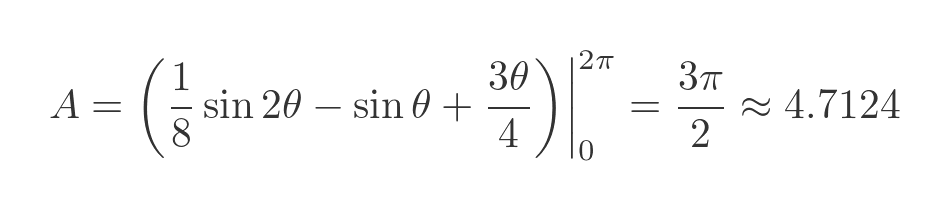
This is the area under a cardioid curve.

Area between curves

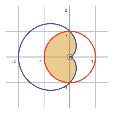
As a final example, we will look at the area between two polar curves. The red curve is the unit circle, the blue curve is a cardioid curve. The cardioid curve has the following equation (from the previous example):

We will be finding the yellow area between the two curves:

In any problem like this, it is first useful to know where the two curves intersect. For a polar coordinates problem, we need to find the intersection in terms of r and θ. In this case, since the circle always has a radius of 1, the intersections will take place wherever the cardioid curve has a value of 1. This occurs when:

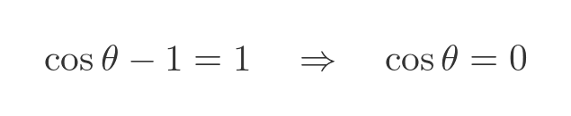
This happens when θ is equal to π/2 or -π/2. Both of these points are on the y-axis. As this diagram shows, the area of interest is divided into three parts by the y-axis:

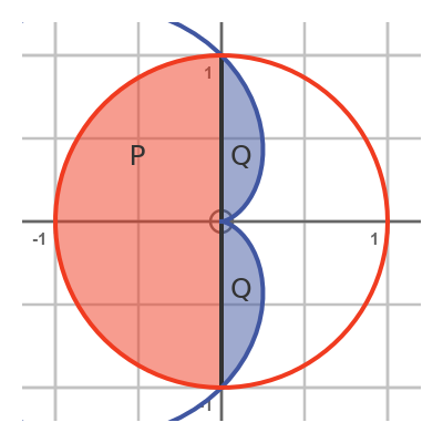
The area P on the left is part of the circle, and in fact, it is exactly half of the semicircle. From before, the area of the full circle is π, so P = π/2.

The two areas Q are both part of the cardioid shape. The areas are identical because a cardioid shape is symmetrical. We only need to calculate the top Q area is the integral of the cardioid function between 0 and π/2. Using the previous formula for the cardioid area:

We already know that the formula is zero when θ is zero, so we just need to calculate its value at π/2:

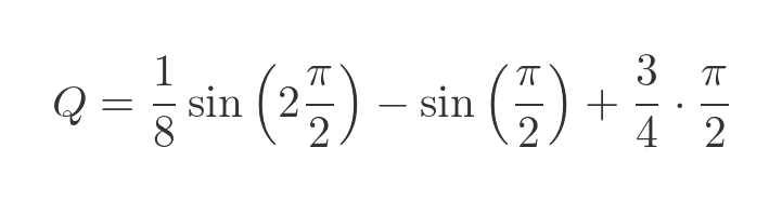
Since the sine of π is 0, and the sine of π/2 is 1, this simplifies to:

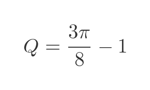
The total area between the two curves is:

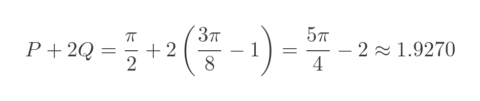
Again this result looks plausible from the diagram.

See also

• Standard curves in polar coordinates
• Polar curve constant r
• Polar curve constant theta
• Polar curve r proportional to theta