Partial fraction decomposition

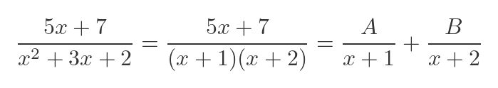
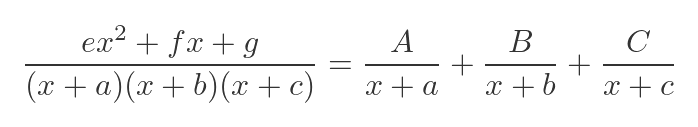
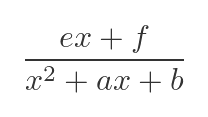
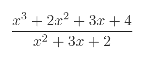
Suppose we have an expression of the form:

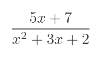
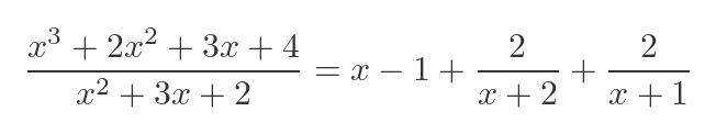
This expression can be written as:

The two expressions are the same function - this can be seen easily by combining the two fractions in the second expression:

Partial fractions

The version with two fractions is often more useful. For example, it is easier to integrate the two simple fractions rather than the original fraction involving a quadratic. This technique is also useful for evaluating Laplace transforms.

This is called a partial fraction decomposition, or sometimes a partial fraction expansion. This technique can be used to simplify functions of the form:

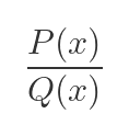
where P and Q are polynomials, and P is a lower order polynomial than Q.

In this article, we will look at several examples of how partial fractions work. We will look at several patterns that work where Q is a polynomial of order 2 or 3 (ie quadratic or cubic), and also see how to extend these patterns further.

Finding the partial fractions

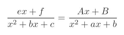
We have verified that the two expressions above are equivalent, but how do we find the partial fractions? Well, we use a set of standard patterns. The first pattern is this one:

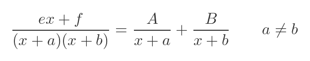
Here, a, b, e and f are coefficients of the expression we are trying to decompose. A and B are two numbers that we need to find. For expressions matching the form on the LHS, each term in the denominator gives one of the terms on the RHS.

Taking our original example, if we factorise the quadratic, it matches the pattern (with values 1, 2, 5, 7 for a, b, e and f):

We need to find A and B. The first step is to multiply through by the LHS denominator, and simplify:

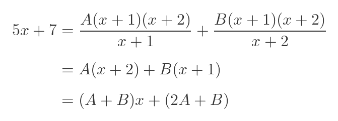
Now, of course, the x terms on both sides must be equal, and the constant terms must be equal, so we have a pair of simultaneous equations in A and B:

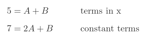
These can be solved quite trivially to give A = 2 and B = 3. This gives the result we saw in the previous section:

One final point to note is that the values of either e or f can be zero. For example, if e is 0 and f is 2, the polynomial P is just a constant value 2:

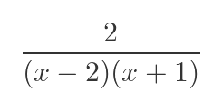
This can be solved in exactly the same way as the previous case.

Adding an extra term

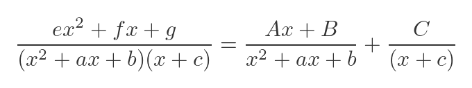
We can extend this pattern by adding an extra term, x + c, to the denominator on the LHS. Here is what we get:

We will assume a, b and c are all distinct values. Notice what has happened here. The extra term x + c in the denominator on the LHS has added an extra term in the sum on the RHS. Notice also that the numerator is now allowed to be a quadratic (because the denominator is cubic). It doesn't have to be a quadratic, because the value e is allowed to be 0, but it can be quadratic.

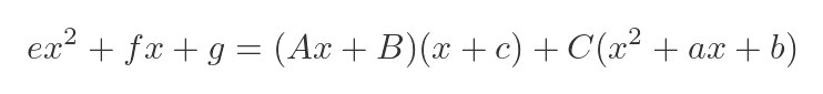
We can solve this, again, by multiplying through:

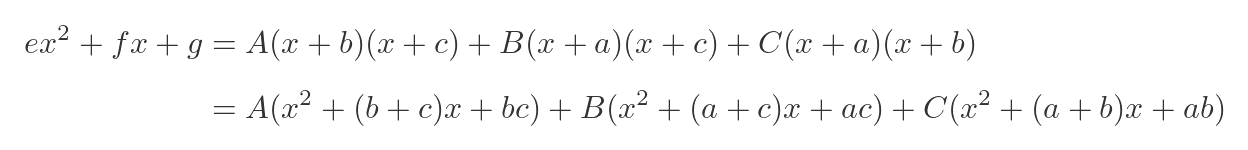
If we expand out the brackets in each term on the RHS, we can then equate x², x, and constant terms. This will give us three simultaneous equations in A, B, and C. We won't do this in detail as it follows the same pattern as before, it is just a little more long-winded. But, essentially, we can find A, B, and C based on the values a to g on the LHS.

The case when a = b

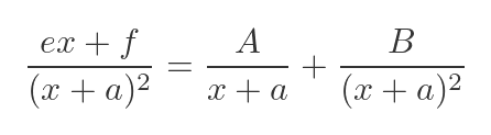
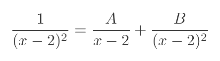
Going back to our original equation, we use a slightly different pattern when a = b:

We will use this example:

As before, we multiply through by the LHS denominator and simplify:

Again, this reduces to a pair of simultaneous equations:

A is 1, so clear;y B is 3. This gives us the following partial fraction decomposition:

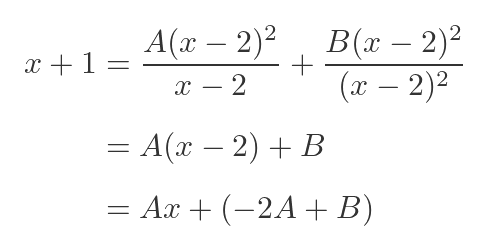
One thing to notice here is that this decomposition isn't useful if e is 0 (so the numerator is just a constant). For example, if e is 0 amd f is 1, we have:

Comparing both sides, it is clear that A (because there is no equivalent term on the LHS), and B must be 1 to match the term on the LHS. So the equation becomes:

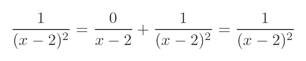
So the decomposition is identical to the original. However, this pattern can still be useful for partial fractions with more terms in the denominator.

Adding an extra term when a = b

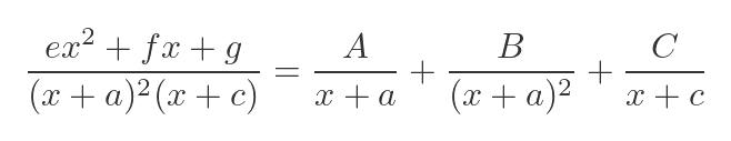
What happens if we add an extra term to the denominator in this case? If the new term has a distinct value, c, it behaves in the same way as the previous example:

The extra term on the LHS adds an extra term to the sum on the RHS.

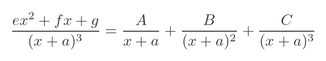
Here is the case where a = b = c. This time, we add an extra term in x + a cubed:

We now have a set of rules for different cases where the LHS denominator can be fully factored into linear terms. We have seen how to extend the simple case in various ways, so we should be able to handle any situation by breaking it down into one or more of the cases we have looked at. There is just one more case to consider.

The case when the denominator cannot be factored

A final case is where the denominator is a quadratic that cannot be factored:

Here is an example. We can't factor the quadratic because b² is less than 4ac:

The pattern we use in this case is:

Now you might notice a problem here. The solution has A = e and B = f, which then makes the RHS identical to the LHS. This type of fraction cannot be decomposed into partial fractions. However, the identity above is still useful to know when we add an extra term.

Adding an extra term when the denominator cannot be factored

So, let's look at the previous example where the denominator was a quadrilateral that could not be factored. But this time we will add an extra term to the denominator:

If we multiply through, we get this:

In the earlier case, we found that A and B were equal to e and f, so no simplification was possible. But in this case, we can find A, B, and C in terms of the known values, so we can obtain a useful simplification.

Case of higher order numerator

In all the cases above, the denominator has a higher order than the numerator. But what happens when the order of the numerator is greater than or equal to the order of the denominator? Here is an example:

The way to handle this is to apply polynomial long division. We won't cover that here, but if we divide a polynomial by another polynomial of lower order, we obtain a quotient (which is a normal polynomial) and a remainder. The remainder is a polynomial that always has a lower order than the divisor. Here is the result of the division:

The quotient is x -1 and the remainder is 4x + 6 (which still needs to be divided by the divisor, as shown). We can then decompose the remainder in the usual way:

This, again, results in a sum of simpler terms.

Related articles

• Factorials
• Prime factors of a number
• Lowest common multiple (LCM) of two numbers
• Greatest common divisor (GCD) of two numbers
• Trinary numbers
• Root 2 is irrational - proof by the carpets theorem
• Root 2 is irrational - proof by prime factors
• The golden ratio
• Algebraic and transcendental numbers