Introduction to Laplace transforms

A Laplace transform is a type of integral transform that acts on functions. It transforms a function of variable t into a different function of a different variable, s.

We can write this as:

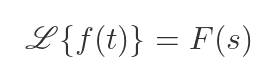
In this equation, the stylised L represents the Laplace transform. We use braces to indicate that the transform accepts a function, rather than a value, as its argument. f(t) is our original function in t, and F(s) is the transformed function in s.

Why is this useful? Well, the Laplace transform has a special property. If f(t) happens to be part of a differential equation, ie it contains terms that are derivatives with respect to t, those terms become simple multiplicative terms in F(s).

We can often simplify F(s), then perform an inverse Laplace transform to find the solution to the differential equation in t.

In this article, we will learn how to:

• Derive the Laplace transforms of a simple function
• Find the Laplace transform of a composite function
• Find the Laplace transform of the derivative of a function
• Invert a Laplace transform

What is the Laplace transform

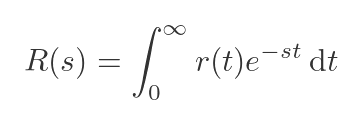
First, we need to define the Laplace function. For some function f(t), the Laplace transform is defined as:

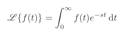
Notice that this is a definite integral in t (that is, it is an integral between two fixed boundaries, 0 and ∞). This means that the result of the integral doesn't depend on t. However, it can depend on s. We will look at this in more detail in the next section.

Notice also that this is an improper integral, because the upper bound is infinite. This means that, when we evaluate the integral, we need to check that it converges to a finite value.

Laplace transform of t

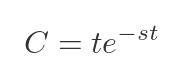
As a simple example, let's take a simple function:

If we plug this into our formula for the Laplace transform, we get the following integral:

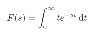
So the value of F(s) is equal to the total area under the curve C, where C equals:

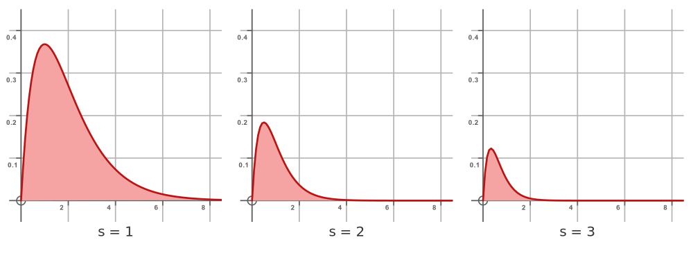
As we change s, the shape of the curve changes, so the area under the curve changes, which changes the value of F(s). This is shown for several different values of s here:

Solving the integral

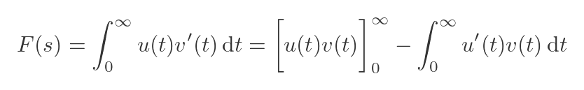
To find F(s), we need to solve the integral above. Since it is an integral of the product of two functions, we might try integration by parts. The general formula is:

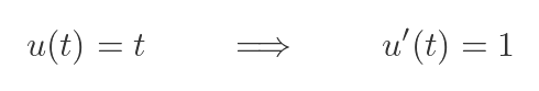
We will use u(t) = t, so the derivative is 1:

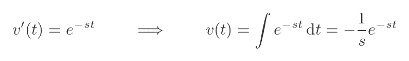
This means that v'(x) is the exponential term. We can find v by integrating this term. It is a standard integral (described here):

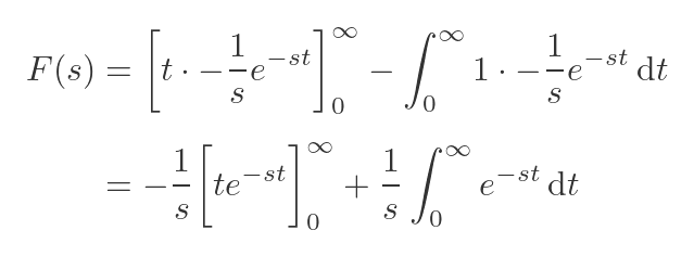
Substituting these terms back into the original integration by parts, and simplifying, gives:

We have two terms in t that we need to evaluate. The first is the u(t)v(t) term in square brackets:

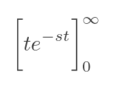
When t is 0, the exponential term is 1, so the whole expression is 0. When t tends to infinity, provided s > 0, the exponential term will tend to zero because the exponent will tend to -∞. The t term will tend to ∞. We won't prove it here, but because the exponential term tends to zero faster than the t term tends to infinity, the expression as a whole tends to 0 as t tends to ∞. This means that the square bracket evaluates to 0.

Next, we need to look at the integral term. We already know this integral from when we integrated v'(t):

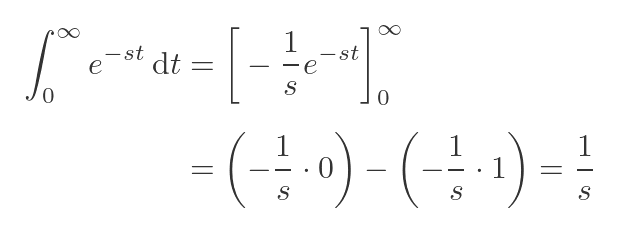
Again, we specify that s > 0 so that the exponential term tends to 0 as t goes to ∞. We will see what this restriction means in a later article. We can substitute the previous two results into our expression for F(s), giving quite a nice result:

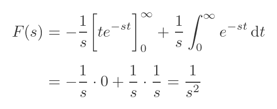
Since we are assuming that s > 0, we don't need to worry about dividing by s in the formula.

Here is the graph of the Laplace transform F(s) of the function f(t) = t:

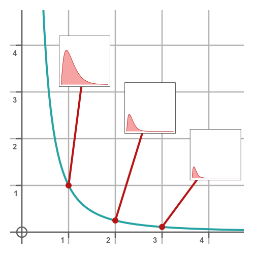
To recap, each point on the main graph F(s) is equal to the area under the curve C for that particular value of s. The small graphs show the curve C for s values of 1, 2 and 3.

In principle, we can find the Laplace transform of any function by evaluating the integral for that function. This has been done for many different functions, and we will look at some other functions in a later article. There are tables of Laplace transforms readily available online.

Laplace transforms of a linear combination of functions

Suppose we have two functions, p(t) and q(t), and we happen to know their Laplace transforms P(s) and Q(s). Now let's consider a function r(t) that is a linear combination of p and q:

Here, a and b are constants. It turns out that the Laplace transform of r(t) is given by:

This rule allows us to simplify more complex functions, so it allows us to easily apply Laplace transforms to a far larger set of functions.

Proof of linear combination rule

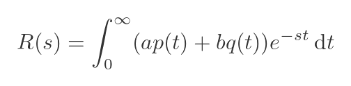
It is quite easy to prove the rule, simply from the definition of the Laplace transform:

We can replace r(t) with the expression in p and q:

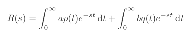
The sum in the integral can be split into two separate integrals:

a and b are constants, so they can be moved outside the integral:

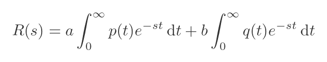
Now the integral in p(t) is the definition of P(s) (and similar for q), so:

This can easily be extended to include three or more terms.

Laplace transform of derivative

We are going to jump ahead a little bit now, to illustrate the feature of Laplace transforms that makes them special (and extremely useful). We will find the Laplace transform of the derivative of a function f(t). And the cool thing is that the Laplace transform only depends on F(s). We can find the Laplace transform of the derivative of a function without differentiating the function!

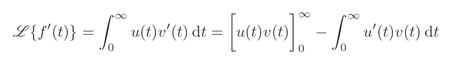
Let's start with the normal Laplace transform, but applied to f' rather than f:

We will solve this using integration by parts, just like the earlier example:

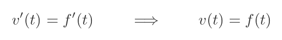
This time it will be convenient to use the first part, f'(t) as v'(t), because then v(t) is just f(t):

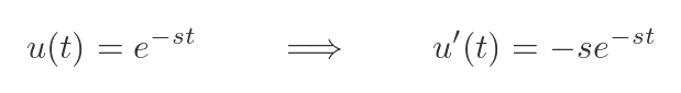
So we then need to use the exponential term as u(t). That is fine, because it is easy to differentiate an exponential:

Putting this all together gives:

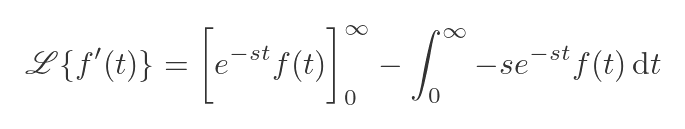
Notice that the RHS only consists of terms in f, there are no terms in the derivative of f. We will start by expanding the first term:

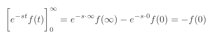
As this is just an overview, we can play a bit fast and loose with the limits. The first expression is the exponential of -∞ (assuming s is positive, as usual) multiplied by f(∞). So the exponential rapidly goes to zero. If we assume the function f doesn't zoom off to infinity faster than the exponential goes to zero, the first term will be zero. In the second expression, the exponential has an exponent of 0, so its value is 1. So the whole thing reduces to -f(0).

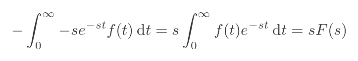
Here is the second expression. We can tidy it up by cancelling out the two negatives and bringing the s outside the integral sign. This gives us s multiplied by the Laplace transform of f:

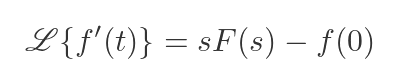
So the Laplace transform of the derivative of a function (any function!) is:

Inverse Laplace transform

We know that the Laplace transform can find F(s) given f(t):

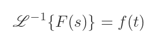
The inverse transform reverses this procedure. We use it to find f(t) given F(s):

One common use of Laplace transforms is to solve differential equations. As we saw previously, the Laplace transform of the first derivative of f(t) depends only on s and F(s). The same is true of the second derivative and higher derivatives. The typical process for solving a differential equation is:

• Apply the Laplace transform to express the differential equation in terms of F(s) and s.
• Solve for F(s). This will give an expression in s.
• Apply the inverse Laplace transform to convert F(s) to f(t)

Tables are available that list the Laplace transforms of many common functions. Finding the inverse Laplace transform is usually done by manipulating the expression until it is in the form where all the elements are known Laplace transforms, then the solution can be found from the table.