Convolution - moving average filter

Convolution can be quite a difficult concept to get to grips with. This article uses a simple application, a moving average filter, to help visualise the process.

An example signal

Here is a function that represents our "signal". Convolution, of course, is a mathematical process that operates on mathematical functions, but in many practical applications, those functions might represent physical signals. For example, this function might represent a sound:

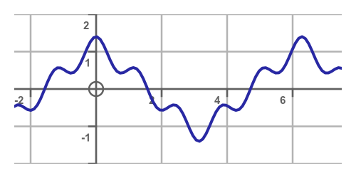
We might see this signal on an oscilloscope measuring a voltage in an electronic amplifier that will eventually be converted to sound waves by a speaker. Although in this case, the signal shown has an oscillation period of several seconds, so humans would not detect it as a sound.

Since this is a time-varying signal, the horizontal axis represents time, t, rather than x. We will call the function above f(t).

A simple filter

Let's suppose we wanted to modify this signal by smoothing out some of the smaller bumps in the function. This would have the audible effect of increasing the bass and decreasing the treble, sometimes called a lowpass filter.

One simple way to do that would be a moving average filter. In this type of filter, the output consists of the average value of the signal over a certain period of time. As an example, we will take the average value of the signal for the previous 1-second period.

In the graph below, the top curve shows the input function from earlier. The bottom graph shows the filtered function, which we will call w(t). To find the value of w(t) at point a (when t is 0), we simply need to find the average value of the input function between t values of -1 and 0. This region is shown shaded on the top graph. It is the average value of the shaded region on the left, and is a positive value.

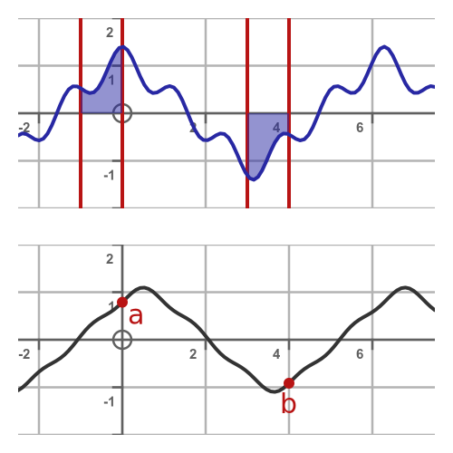
Point b on the lower graph (when t is 4) represents the average value of the function between t values of 3 and 4, and this time it is a negative value.

Of course, we can find the value of the lower graph for any value of t. It is simply the average value of the top graph over the range (t - 1) to t.

Calculating the value of w(t)

We can calculate the value of $w(t)$ for any value of $t$ using integration. The average value of f(t) is given by the area under the curve, divided by the width of the region. In our case, the width of the region is 1, so the average value is:

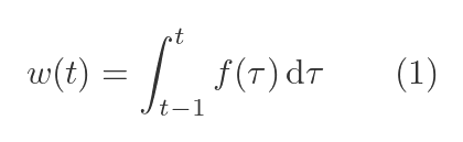
We have used the Greek letter 𝜏 (tau) as the variable of integration, but notice that w is a function of t, not 𝜏. For example, when t is, the integral will find the area under the curve between -1 and 0, corresponding to point a above. When t is 4, it will find the area between 3 and 4, corresponding to point b, and so on.

Using a function instead of varying the limits

In the integral above, we change the limits of the integral to determine the region that we are interested in (for example, using limits of 3 to 4 to find the average value over that region). But there is an alternative method, illustrated by this graph:

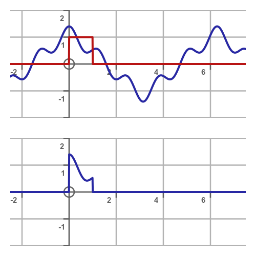
The top graph shows our original function f(t) in blue, and a new function g(t) in red. g(t) is defined by:

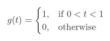
It is a gating function that has value 1 between 0 and 1, and 0 everywhere else.

The bottom graph shows g multiplied by f. It has the value of f for t between 0 and 1, and 0 everywhere else. The useful thing about this function is that we can integrate it from -infinity to +infinity and get the same result as we would get by integrating for 0 to 1 (because the function is 0 outside that range). So we can write w(1) like this:

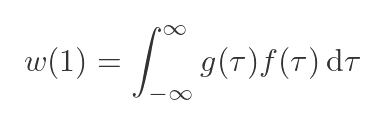
Notice that this is w(1) rather than w(0) because the range starts at 0 and ends at 1. We will address this later.

Now let's look at this graph:

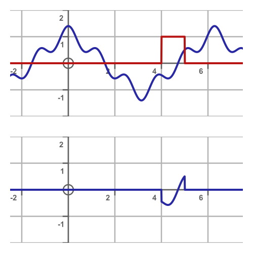
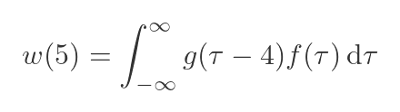
The red function is similar to g(t), but shifted by 4 along the time axis. We will call this new function gs. When we multiply gs by f, we get a new function that is equal to f when t is between 4 and 5, but 0 everywhere else. The integral of gs times f is:

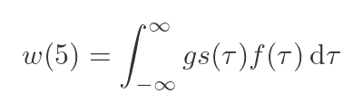
This integral, of course, gives us w(5). Now we can simplify this further. We know from elementary mathematics that we can shift a function horizontally by subtracting a constant from its argument. In other words, we can write gs(t) (ie g(t) shifted by 4) as g(t - 4). So we can write:

And in general, we can say that:

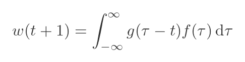
Just like our original equation (1) above, this is a function of t. But this time t is part of the integrand rather than being part of the integral limits, which generally makes things easier, as we will see.

The equation above is the basis of a process called convolution, although we need to do a bit more work to get to the final definition.

Improving the formula

There is a small problem. When we plug some value t into the integral, we end up with w(t + 1). Now this might seem like a very minor problem. Perhaps we could just add a 1 into the integrand as a fudge factor to make it all work?

Unfortunately, it isn't that simple. The reason the function is shifted by 1 is that we happen to be using a moving average filter with a width of 1. If we had chosen a width of 2, a fudge factor of 2 would be required. If we had chosen to use a weighted average rather than a gated average, we might need to use some other value.

There is a simple fix, but it leads to an aspect of convolution that people often find confusing. Hopefully, understanding why it is necessary will make it less confusing.

The top graph below shows g(t), where the function has value 1 from time 0 to 1. The bottom graph shows the function we require, which has a value of 1 for time -1 to 0. How do we transform one into the other?

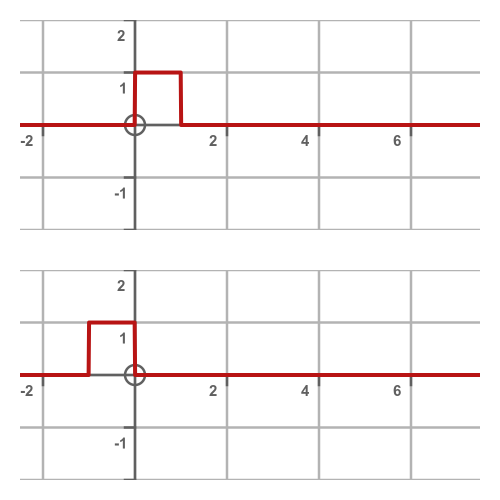
One way would be to shift the function to the left by one second. That would be our fudge factor, mentioned above. But we don't want to do that, because different functions might require shifting by different amounts.

The alternative way is to mirror the function, horizontally, about the y-axis. This operation will always lead to the falling edge of the function being at 0, no matter how wide the raised region of the function is. This is what we will do, and it is actually built into the definition of the convolution integral.

An advantage of this technique is that it is very easy to flip a function about the y-axis. We simply need to negate the argument. For any function g(t), the function g(-t) is the same function, flipped about the y-axis.

In our case, our integral is based on g(t - 𝜏), so to flip it we just need to use g(𝜏 - t) instead:

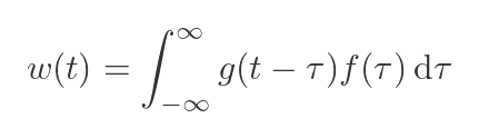
This integral defines the process of convolution.