Complex roots of one

In the Modulus-argument form of complex numbers, we saw how to find the nth root of a complex number, where n is an integer. We saw that, for any non-zero complex number, the number of nth roots is exactly n.

In this article, we will look at the special case of the nth roots of the value 1.

One as a complex number

Any complex number z can be expressed in modulus-argument form, like this:

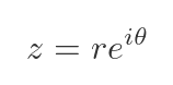
Here r is the modulus of the number, and θ is the argument. For the number 1, the modulus is 1, and the argument is 0, so 1 can be written as:

The square roots of 1

In the real domain, 1 has two square roots: 1 and -1. In the complex domain, this is still true. Here are the two roots on an Argand diagram

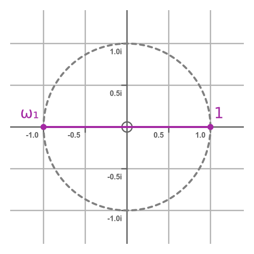
We will use the Greek letter omega (ω) to denote the roots of 1 (other than the value 1 itself). We will use a subscript the different roots. For the square root, there is only one root (other than 1), which we will call ω₁. If we look at this in modulus-argument form, here is what happens when we square 1:

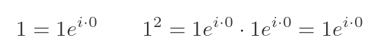
We have just followed the normal rules for multiplying complex numbers - we multiply the moduli and add the arguments. But since the moduli are both 1, and the arguments are both 0, the result is just 1. This is no surprise, we know that 1 squared is 1.

Here is what happens when we square ω₁ (which is equal to -1) in modulus-argument form. The modulus of -1 is 1, and the argument is π, so here is what happens when we square it:

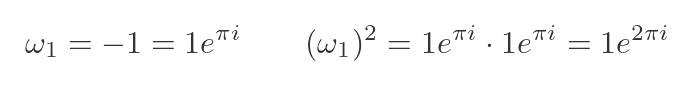
Again, we multiply the moduli and add the arguments. Again, the moduli are both 1. But this time, the arguments are both π, the result has an argument of 2π. Of course, the argument corresponds to the angular position of the complex number, and an angular position of 2π radians (360°) is equivalent to an angular position of 0. So ω₁ squared gives the result 1. Again, this is no surprise, we know from elementary maths that -1 squared is 1.

Looking at this in the complex domain, point ω₁ is rotated by 180° from the positive-going real axis, and when we square it, we rotate it by another 180°, which gets us back to +1.

The cube roots of 1

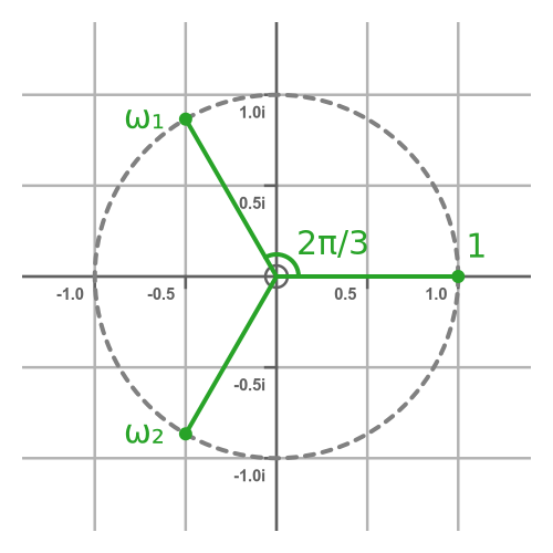
We know that, in the real domain, 1 only has a single cube root, which is 1. If we cube -1, of course, we get -1, so that isn't a cube root of 1. But in the complex domain, 1 has three cube roots. We will call the roots 1, ω₁, and ω₂:

Notice that the ω values depend on which root we are taking. The value of ω₁ for the cube root is not the same as the previous value of ω₁ for the square root.

We won't prove it here, but the three cube roots of 1 are evenly distributed around the unit circle, so the angle between each pair of roots is 2π/3. And, since we know that one of the roots in 1, that means that the other two roots must be at angles 2π/3 and 4π/3.

So ω₁ has modulus 1 and argument 2π/3. Here is what happens when we cube it:

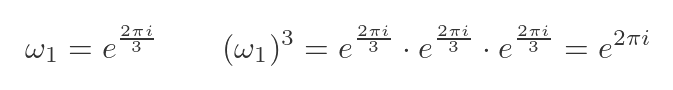
Starting from 1, if we multiply by ω₁ three times, we complete a full rotation of 360°, which gets us back to 1.

(Notice we have removed the factors of 1 from each exponential term. They were shown previously to emphasise that the modulus was 1, but we don't need to continue doing it.)

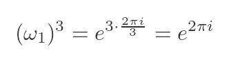
We have found the cube of the exponential term by multiplying three terms together. But there is a simpler way. We can cube an exponential simply by multiplying the exponent by 3:

As we noted. ω₂ has an argument of 4π/3. Here is what happens when we cube it:

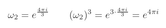
Converting this to degrees, ω₂ has an argument of 240°, when we cube it, we get a total rotation of 720°, which is two full turns. But it still gets us back to 1, so ω₂ is a cube root of 1.

In summary, 1 has three cube roots. They are all on the unit circle, and they are evenly distributed (at 0°, 120° and 240°).

The fifth roots of 1

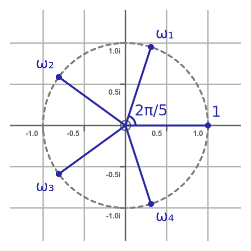
As a final example, we will look at the fifth roots of 1. As you might expect, there are five roots (including 1 itself), evenly distributed around the unit circle, so they are separated by angles of 2π/5 radians (72 degrees). They are labelled here as 1 and ω₁ to ω₄:

If we take ω₁ and raise it to the power 5, we get 1:

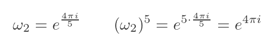
Similar for ω₂ (this time the total rotation is 720°, or two full turns):

Similar for ω₃ (this time the total rotation is 1080°, or three full turns):

And ω₄ follows the same pattern.

The relationship between ω values

We have used ωₖ to represent nth roots of 1, where k takes values 1 to n - 1.

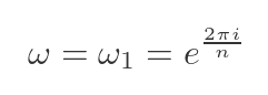
It is useful to define the principal root, ω. The principal root is the root with the smallest positive argument. This means that the principal root is always ω₁.

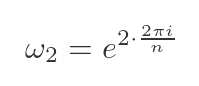
As mentioned earlier, the value of ω₁ (and therefore ω) is different for different values of n. In fact, for any n > 1, ω is given by:

This definition allows us to find an interesting relationship between ω and ω₂. We know that ω₂ has twice the angle of ω, so we can write it by doubling the exponent of ω:

But we also know that squaring ω has the effect of doubling the exponent, so we can do this:

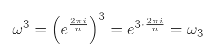
So ω₂ is equal to ω squared. Using the same method, we can also show that ω₃ equals ω cubed:

And in general ωₖ equals ω to the power k:

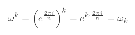
So we have ωₖ = ωᵏ. To reiterate, these two similar looking terms mean very different things. ωₖ is the kth root of 1, but ωᵏ is the principal root of 1, raised to the power k. But they are equal.

AWe can use this define ω₀ as 1:

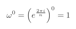
This works because any non-zero value raised to the power 0 is 1.

These results can often be useful in proofs relating to complex numbers.

Related articles

• Complex exponential function
• Complex natural log function
• Complex sine and cosine functions