Complex natural log function

In this article, we will look at the natural log function in the complex domain. We will also briefly look at the concept of branches of a function.

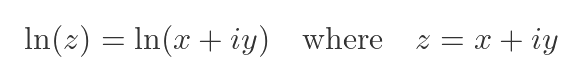
The log of a complex number is:

To understand what this means, we will rely on some of the definitions and properties of the complex exponential function. It might be worth reviewing that article if you are not familiar with complex exponentials.

Logarithm of an imaginary number

In the real domain, we define the natural logarithm to be the inverse of the exponential function (that is, e to the power x). So we have:

Of course, since the exponential function always returns a positive value, the ln(x) function is only defined for positive values of x.

So what is the log of a complex number z? The answer is that it is whatever we define it to be. But we need to make sure we choose a definition that makes sense. A definition that is consistent and useful.

It turns out that a very useful definition is, perhaps, the most obvious one. We simply define the complex log function to be the inverse of the complex exponential function:

Where w and z are complex numbers.

Multiplication using complex logarithms

One important feature of real-valued logarithms is that:

It would be very useful if the same were true for the complex log function. And it is, as we will prove now. First, let's define two complex numbers, z1 and z2, and their logarithms w1 and w2:

Since log and exponential are inverse functions, this implies that:

We can find the product of the two numbers:

We know that, for the complex exponential function, we can find the product by adding the exponents (proved here):

We can take the log of both sides, remembering that log and exponential functions are inverses, so they cancel out:

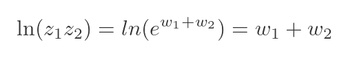
Finally, we can substitute the values of w1 and w2 from the earlier equation:

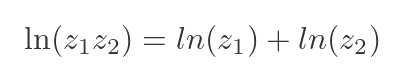
This proves that the addition rule works for the complex log function. Actually, there is a slight caveat here. As we will see in a moment, the complex log function is multi-valued, so we need to be slightly careful. We will look at that in more detail later.

Complex log formula

Now we have defined what we mean by the complex log, but how do we find its value? In fact, we can do that based purely on our definition. First, we will express z in polar form, using Euler's formula:

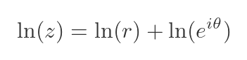
We can take the log of both sides:

Now we have the log of a product of two complex numbers, r and the exponent of iθ. We know from earlier that we can split this into the sum of two logs:

But since log and exponential are inverse functions, the second term can be simplified:

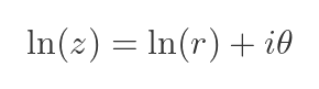
That is it! If we express z in polar form, we can calculate its log. Here is the same formula, but using the modulus and argument of z instead of r and θ:

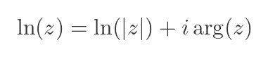
So, the log of z is a complex number whose real part is the log of the modulus of z, and whose imaginary part is the angle of z.

The logarithm is a multi-valued function

For any z (other than 0), the log of z has more than one value. This might seem strange, but in fact, there are many simple functions that have this property. For example, the square root function. We normally say that the root of 4 is 2. But, of course, we know that -2 is also a root of 4.

Why does this come about? It is because there are two ways of expressing the number 4 as a square. We can say 4 is 2 squared, or we can say that 4 is -2 squared. They are both the same number, 4. But the square root of 2 squared is not the same as the square root of -2 squared.

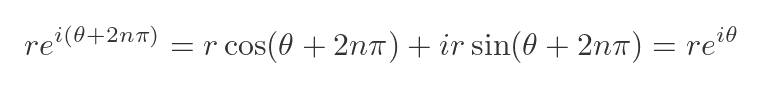
When we express a complex number in polar form, we get a similar effect:

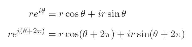
Adding 2π to θ makes no difference to the result of the sine or cosine functions, so both of the complex numbers above have the same value. In fact, adding 2nπ to θ, for any integer n, still gives the same complex number:

However, when we take the log of that number, we get:

This is clearly different for every value of n, so in fact there are infinitely many values for the complex log of z.

How z maps to w

To get a feel for the overall function, it is useful to see how different values of z (the original value) map onto w (the value of ln(z)). As we saw earlier, ln(z) can be calculated as:

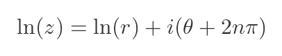
First, we will look at the real part of w. It is given by the log of the modulus of z. On the LHS of the graph below, the inner red circle has a radius of 0.5. It represents all the points where the modulus of z is 0.5.

Since all these points have the same modulus, and the real part of w depends only on the modulus of z, then all these z values map onto w values with the same real part. That is, a vertical straight line, shown on the RHS:

This line is positioned at ln(0.5) on the real axis, which is about -0.6931.

The blue circle has a radius of 1 and defines all the points where the modulus of z is 1. This corresponds to w values with a real part of ln(1), which is zero. So the blue line on the RHS is positioned at 0 on the real axis.

AS the circles get bigger, the corresponding line in the w domain moves to the right (the real part of w increases). But since the increase is logarithmic, the lines get closer together (even though the circles in z are equally spaced).

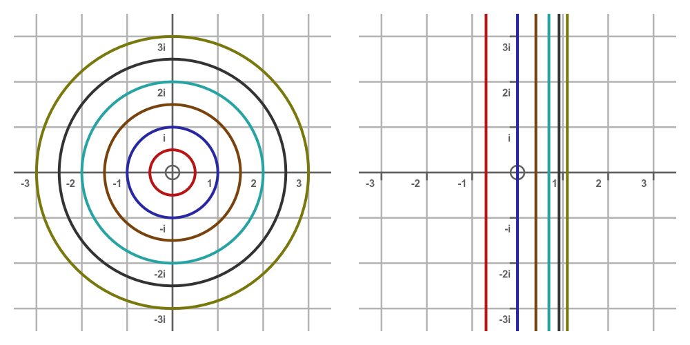
Now let's look at the imaginary part of w. From the equation, this is equal to θ, the argument of z. This means that all z values with the same argument will correspond to w values that have the same imaginary part.

For example, the red radial line on the LHS below represents all the z values where θ is 0. This maps onto the solid red line on the RHS that crosses the imaginary axis at 0:

The blue line on the LHS (making an angle of 60 degrees with the +ve x-axis) represents all values of z with an argument of π/3. This corresponds to w values with an imaginary part of π/3. This is the solid blue line, just above the x-axis, in the RHS. The other solid lines represent different values of θ.

But remember, of course, that we can add multiples of 2π to the argument of z without changing its value. So the blue line on the LHS doesn't just represent an argument of π/3, it represents all arguments of (π/3 + 2nπ) for all integer n.

For example, if n is 1, the argument is (π/3 + 2π), which is about 7.3304. This is shown by the dashed blue line on the RHS that crosses the real axis at that point. If n is -1, the argument is (π/3 - 2π), which is about -5.2360. This is shown by the dotted blue line on the RHS that crosses the real axis at that point.

There are further lines for n of 2, 3 ... and for n of -2, -3 ... carrying on forever in each direction. This is a further illustration of the multivalued nature of the complex logarithm.

Principal values

In the square root example, we know that the square root os 4 can be ±2, but we define the square root function to always return +2, so that it is a single-valued function. If we want to consider both possibilities, we must explicitly state that.

A similar concept exists for multivalued complex functions, but it works slightly differently. The arg function represents all possible values of θ, that is, θ + 2nπ for all integer values of n.

We use the special function Arg (like arg but with a capital A) as a function that only returns the principal value of θ. The principal value is the value that is greater than -π and less than or equal to π.

In addition, we define a function Ln that calculates the complex log based on the principal value of θ. So in the previous graph of the imaginary part of w, if we used Ln(z) rather than ln(z), we would only get the solid lines, not the dashed or dotted lines.

Interpreting the mapping as a change of coordinates

We can combine the previous two graphs to show the complete picture of how different points map from z to w when we apply the complex log function.

So any point in z can be mapped onto its equivalent point in w like this:

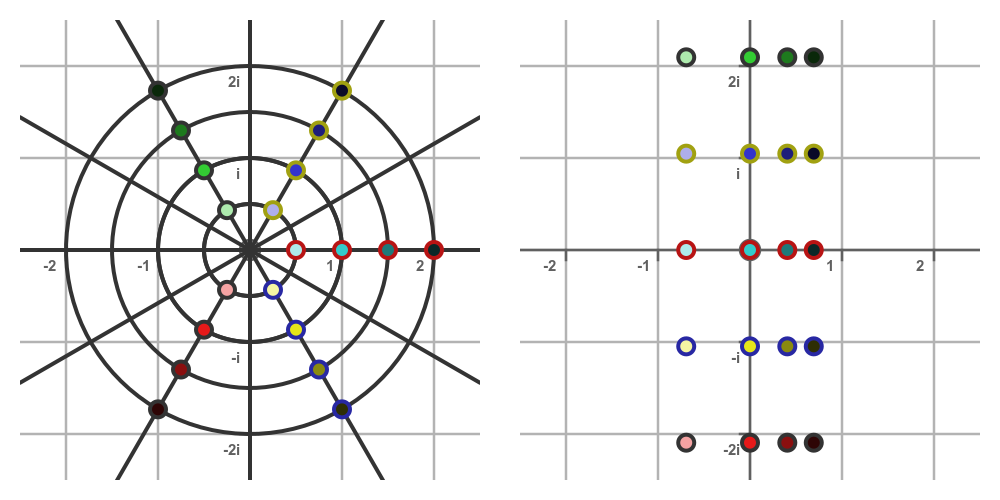
The LHS shows some different z values. The basic colour and outline of each dot indicates its angle, arg(z). For any given angle, the basic colour is the same, but gets darker as the modulus, |z|, increases.

The RHS shows how these values are mapped onto equivalent w values:

• All points with the same arg(z) are mapped onto the same horizontal line (because w has the same imaginary part).
• All points with the same |z| are mapped onto the same vertical line (because w has the same real part).

Heatmaps of complex logarithm

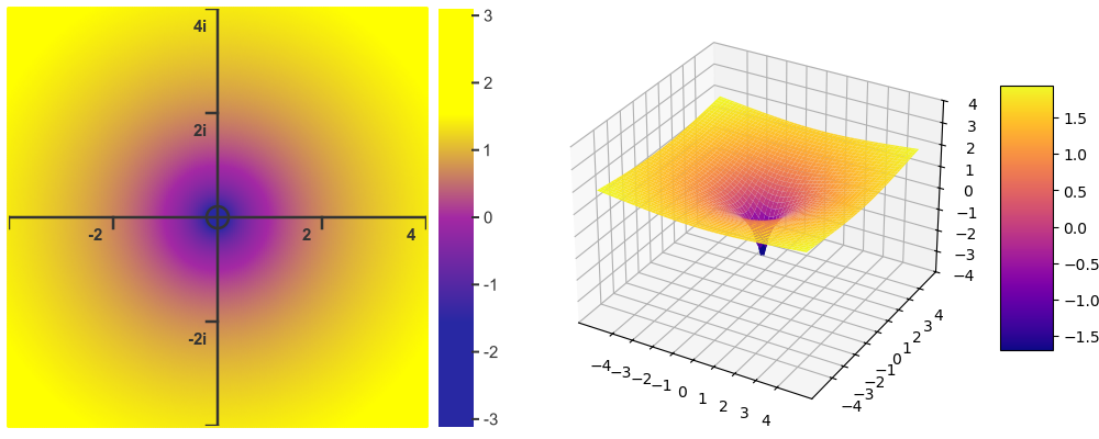
Here is one final way to visualise the function, using heatmaps and 3D plots. The graph below shows the real part of the function. Since the real part is the log of the distance from the origin, as we approach the origin, the function becomes increasingly negative. This results in a "well" of infinite depth.

This next graph shows the imaginary part of the function:

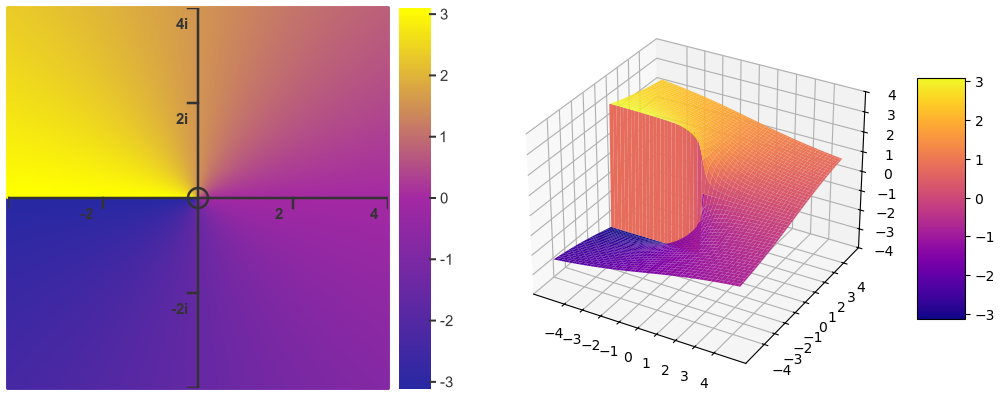
The imaginary part of the function is simply the value of the angle, θ. This makes a spiral shape, as shown. Looking at the negative going real axis of the heat map, we can see a step transition between yellow (representing the value π) and blue (representing the value -π). The 3D plot shows that the function jumps at that point.

This step is called a branch cut. We will cover that in more detail in a future article, so we will only look at it briefly here.

The reason for the step change is that as we approach the cut from the yellow side, θ is increasing towards π, but as we approach the cut from the blue side, θ is decreasing towards -π.

Remember that the function is multivalued. We have decided to only show values for -π to π. If we look at the 3D plot, starting from the blue area, as θ increases, the function spirals up through the magenta area to the yellow area.

For the multivalued function, rather than jumping back to the blue area, the graph would continue spiralling upwards, forever.

Related articles

• Complex exponential function