L system trees and ferns

In the L Systems article we learned that an L System is a grammar-based system for simulating biological growth. It uses the grammar rules to simulate each stage of growth. It then applies some drawing rules to the resulting string, using simple turtle graphics, to create an image.

Previously we illustrated this with a simulation of algae, and also the fractal Koch curve. This time we will expand this to simulate tree and fern-like structures.

Binary tree

We will start by creating this binary tree. It isn't a very realistic tree, but it introduces a new feature that many plant-like structures possess - branching:

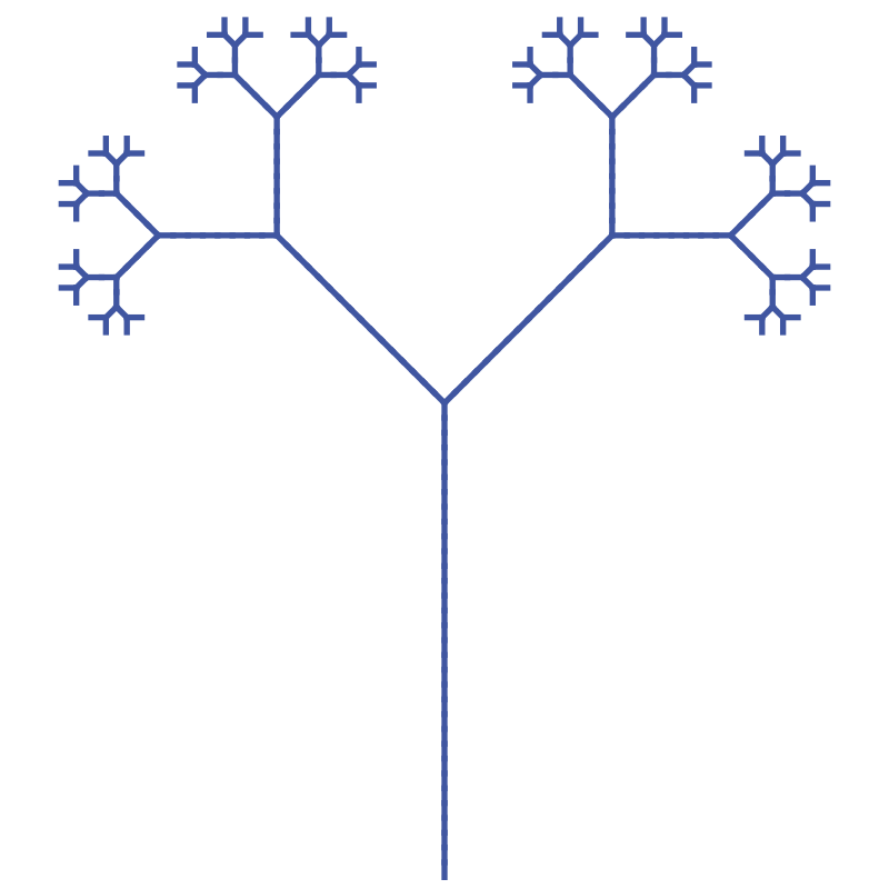
The technique used to create this tree will be used later to create a realistic fern.

Rules for the tree

The tree has an alphabet of 6 symbols:F, G, +, -, [ and ]

Here are the grammar rules for the tree:

• F becomes G[+F]-F
• G becomes GG
• + becomes +
• - becomes -
• [ becomes [
• ] becomes ]

The axiom is F.

Here are the drawing rules:

• Initially the turtle is at position (0, 0), pointing upwards (ie along the positive y-axis).
• F makes the turtle move forward by a 1 unit, drawing a line as it goes.
• + makes the turtle turn to the left by 45 degrees, without moving.
• - makes the turtle turn to the right by 45 degrees, without moving.
• [ pushes the current turtle position and direction on a stack, without moving the turtle.
• ] pops a previous turtle position off the stack, and moves the turtle to that position and direction without drawing anything.

The [ and ] symbols allow us to draw two different sub-structures that branch from a single point, as we will see.

Iteration 1

After one iteration, the initial F will be replaced with G[+F]-F. This string represents the following drawing instructions:

• Forward 1 unit (in the upwards direction)
• Push current position
• Left 45 degrees
• Forward 1 unit
• Pop and restore the previous position and direction
• Right 45 degrees
• Forward 1 unit

That creates a shape like this:

It is worth looking at this in a bit more detail to see exactly how it is drawn. Here is a diagram:

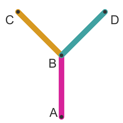
Here is the sequence. It is the same as the sequence described above, but repeated in terms of the actual drawing:

• Start at position A, facing upwards.
• Move forward one unit to B (magenta line).
• Push the current position and direction.
• Turn 45 degrees left and move forward one unit to C (yellow line).
• Pop the previous position and direction. The turtle is now back at B, pointing upwards.
• Turn 45 degrees right and move forward one unit to D (cyan line).

We will call this a Y shape when we refer to it later.

Iteration 2

This time we apply the rules to the string G[+F]-F. This gives a new string:

GG[+G[+F]-F]-G[+F]-F

Which looks like this:

To understand how this works, we will use the same colours as before:

What has happened here? Compared to iteration 1:

• The upright stalk, in magenta, was represented by a G previously. It has doubled in size to become GG.
• The left arm of the tree, in yellow, was represented by an F previously. It has been replaced by a brand new Y shape.
• The right arm of the tree, in cyan, was also represented by an F previously. It has also been replaced by a brand new Y shape.

Notice that the second iteration is bigger than the first. L systems model plant growth, so they get bigger at each stage,

Iteration 3

This time we apply the rules to the string GG[+G[+F]-F]-G[+F]-F. This gives a new string:

GGGG[+GG[+G[+F]-F]-G[+F]-F]-GG[+G[+F]-F]-G[+F]-F

Which looks like this:

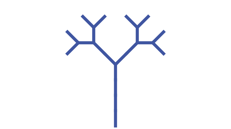
To understand what is going on we can think of the tree as being made up of twigs and branches. Every line in the tree is a branch except the small lines on the edges of the tree, which are twigs. In this diagram, the branches are in magenta and the twigs are in yellow:

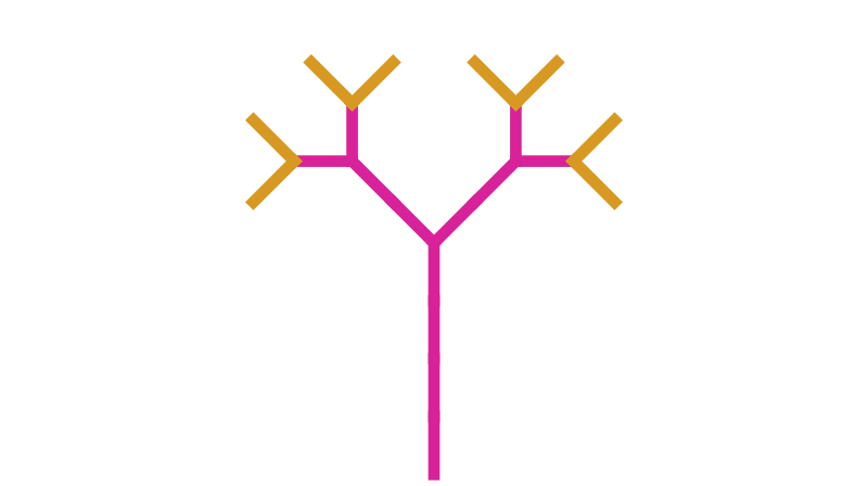
If we look carefully at the string, we can see that every branch is represented by a G symbol (or a sequence such as GG, GGGG, etc). Every twig is represented by a single F.

So we can now understand exactly what happens on each iteration:

• Every branch doubles in length (because each G becomes GG).
• Every twig is replaced by a Y shape (which itself is a short branch with two twigs).

Although the tree is not particularly realistic, the way it grows is fairly similar to how a real tree grows. Existing branches get bigger, and small new branches appear.

After three more iterations, we get the tree we saw at the start of the article. Note that the original illustration is scaled down by a factor of four compared to the first few stages, otherwise it would be too big to fit the page.

A realistic fern

We can make a far more realistic plant by making a few tweaks to the parameters above.

First, we change the rule for F:

• F becomes G+[[F]-F]-G[-GF]+F

This is a slightly more complex rule that contains four F terms that will branch each time.

Next, we change the drawing rule for + and - to turn by 20 degrees rather than 45 degrees. This causes the branches to overlap more, which is a bit more realistic.

Also, we change the colour to green.

Iteration 1

After one iteration, the initial F will be replaced with G+[[F]-F]-G[-GF]+F. That creates a shape like this:

The string that constructs this shape contains four F and three G symbols. But the shape itself only appears to contain 6 line segments.

So what is going on? Actually, it is something quite subtle. This diagram shows the segments coloured as twigs (yellow) or branches (magenta):

The segment coloured in black is a twig and a branch that are both in exactly the same place. In this iteration, we can't tell them apart, but in the next iteration the branch will grow longer and the twig will branch out. The effect simulates a new branch growing out of an old branch, as some plants do, which adds to the realism.

Iteration 2

On the second iteration, the string G+[[F]-F]-G[-GF]+F will be replaced with:

GG+[[G+[[F]-F]-G[-GF]+F]-G+[[F]-F]-G[-GF]+F]- GG[-GGG+[[F]-F]-G[-GF]+F]+G+[[F]-F]-G[-GF]+F

That creates a shape like this:

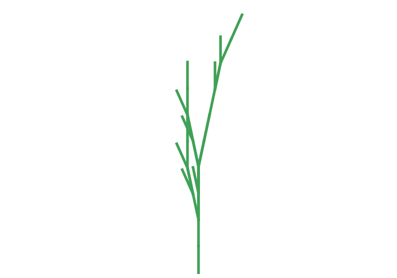
This is a more complex shape than the second iteration tree because the fern contains four F symbols that branch out, rather than just two in the case of the tree. Also, because of the smaller angle, some parts overlap each other.

Later iterations

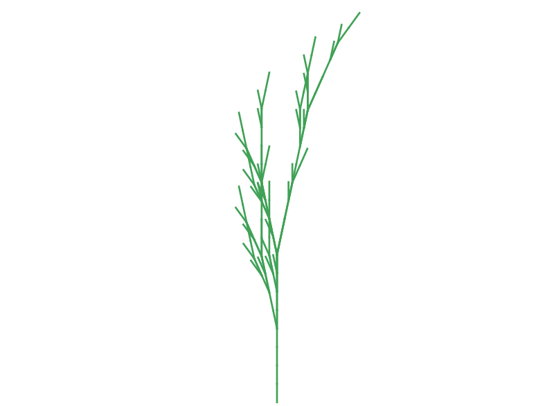
Iteration 3 looks like this:

By the sixth iteration, we have something that looks quite convincing (this image is a twelfth of the scale of the previous iterations):

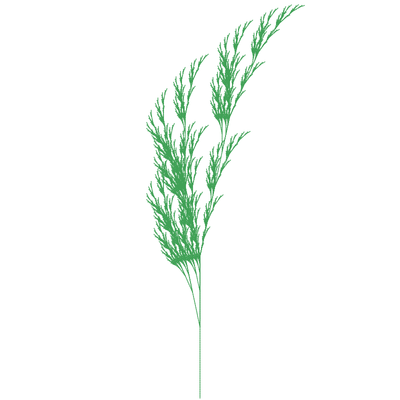
This is all created with a simple, fixed set of rules. There is scope for variation by changing the rules and the branching angle. There are also more advanced techniques where the rules are subject to random variations, or where the rules vary in other ways.

See also

• L system Koch curve