Continuous uniform distribution

Here is a spinning wheel, that has a circumference exactly 1 metre. We will perform an experiment where we set the wheel spinning, and then stop it at a random time. The outer edge of the wheel has distance markers around its edge, showing the distance of that point around the circumference from the zero point. There is also a fixed pointer next to the wheel:

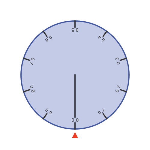
When we randomly stop the wheel, we will measure the position of the fixed pointer on the wheel circumference:

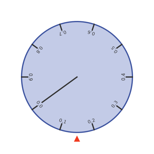
We will call this value X. In the example above, the wheel happens to have randomly stopped where X is about 0.15 (ie it is 15cm from 0.0 on the circumference). What do we know about X?

Continuous random variables

We call X a continuous random variable. Random means that its value cannot be predicted, although there are still certain things we know about X. Continuous means that it can take any value.

This makes X quite different from, say, throwing a dice. Although throwing a dice is random, we know the result will always be an integer from 1 to 6.

There are a couple of other things we know about the rotating wheel. First, we know that the value must be in the range of 0.0 to 1.0 metres because the circle circumference is 1 metre.

Secondly, we can also make the reasonable assumption that any value of X is just as likely as any other.

Probability

So what is the probability of the wheel stopping at some particular value, for example exactly 0.4? Well, it might seem counterintuitive, but the probability of it stopping on exactly 0.4 is zero. We will look at that in more detail later.

For now, let's accept that for a continuous variable, we can only calculate a meaningful probability that X is within a certain range. For example, we can calculate the probability that 0.3 < X < 0.5. We call the range from 0.3 to 0.5 an interval, and we write it as (0.3, 0.5). The probability that X will be in this interval is a fairly simple calculation:

• The total range is possible X values 1.
• The target range of X has a span of 0.2, ie any value in the interval (0.3, 0.5).
• All possible X values are equally likely.

The range of possible values has a span of 1.0 (0.0 to 1.0) the target range has a span of 0.2, so the probaility of X being in the target range is 0.2/1.0. That is 1 in 5.

Probability density function

We can represent the situation using a probability density function (PDF), like this:

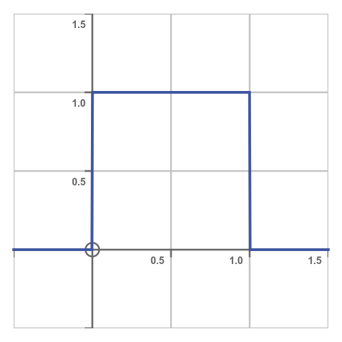
In a PDF, the x-axis represents the value of X and the y-axis represents the probability density. What does probability density mean? It means that a given area under the graph represents the probability that X falls within that area.

This explains the shape of the curve. It is zero outside the interval (0.0, 1.0) because there is zero probability of X taking a value outside that range. And it has a constant value within that range because all values of X within that range are equally probable.

This rectangular shape is a key characteristic of a continuous uniform distribution - an alternative name for it is the rectangular distribution.

What is the height of the rectangle? Well, since X has to be somewhere in (0.0 to 1.0), the probability of being in that interval is exactly 1, so the area under the curve must be 1. This is true of all PDF curves. For example, the area under a normal distribution curve is also 1. In our case, since the rectangle has a width of 1 and an area of 1, its height must be 1.

Probability of X between two values

How do we use the PDF to calculate the probability that X is in the interval (0.3, 0.5)? We need to find the area under the curve over that interval, shown here:

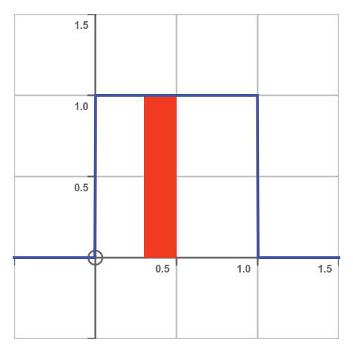
The red rectangle has a height of 1, a width of 0.2, and therefore an area of 0.2. So the probability of X being in (0.3, 0.5) is 0.2.

It is worth noting that (0.3, 0.5) is an open interval - this means it does not include the endpoints 0.3 and 0.5, so it represents the range 0.3 < X < 0.5. The alternative, [0.3, 0.5], is a closed interval which does include the endpoints, so it corresponds to 0.3 ≤ X ≤ 0.5.

Normally in mathematics, this is an important distinction, but in this case it makes no difference. One interval includes the values 0.3 and 0.5, the other does not, but since the probability of X being exactly 0.3 or 0.5 is zero, the two intervals have the same probability.

Fitting the distribution to real data

As a second example, we will look at a village that has a slightly unreliable daily bus service to the nearest town. The bus is scheduled to arrive at 1:30 pm and is never early but can be up to half an hour late. Analysing the arrival times over several months shows the bus is equally likely to arrive at any time between 1:30 pm and 2:00 pm.

Since the probability is zero outside a certain range, and uniform within that range, it can be modelled using a continuous uniform distribution. However, unlike the first example, the permitted range is not zero to one. It is, in hours, 1.5 to 2.0.

For a continuous uniform distribution, we normally call the minimum value a, and the maximum value b. So in this case, a is 1.5 and b is 2.

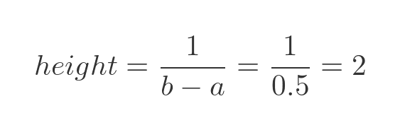
The width of the rectangle is:

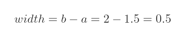
We can also calculate the height of the rectangle. The total area, width times height, must be 1. So the height is:

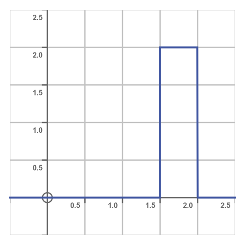
So our PDF looks like this:

We can use this PDF to answer statistical questions. For example, suppose a would-be passenger arrives at the bus stop 5 minutes late. What is the probability that they will miss the bus?

Well, they will miss the bus if the bus arrives between 1:30 and 1:35. This is shown here:

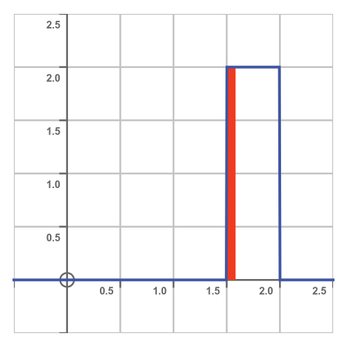
The red area has a width of 5 minutes (1/12 of an hour) and a height of 2, so its area is 2/12 = 1/6. So the probability of missing the bus if you are 5 minutes late is one in six.

The cumulative distribution function (CDF)

The CDF tells us, for any value v, the probability that X is less than v.

In other words, the CDF at v is equal to the area under the PDF up to that point. This diagram shows the PDF on the left and the CDF on the right:

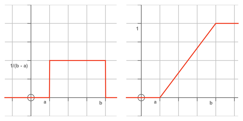
The PDF tells us that every value between a and b is equally likely, and values that are less than a or greater than b are not possible. This means that:

• Every possible value is greater than a, so there is zero probability that X will be less than a. So the CDF for values less than a is zero.
• Every possible value is less than b, so there is a probability of one that X will be less than b. So the CDF for values greater than b is one.

Since the PDF between a and b has the constant value 1/(b - a), the CDF rises linearly from zero to one between a and b.

Key facts about the continuous uniform distribution

The median average value, M, is the midpoint of the distribution. That is to say, X has a 50% probability of being less than M and a 50% probability of being greater than M.

This, of course, is the value of X where the CDF is 0.5. Since the CDF rises linearly from 0 to 1 as X moves from a to b, it follows that the median is the halfway point between a and b:

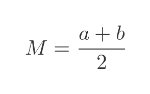
The mean average, µ, is also equal to (a + b)/2, the same as the median. This seems intuitively obvious - the value is equally likely to be anywhere between a and b so you might expect the average to be exactly halfway between them. But a derivation is given below, for those who don't trust their intuitions.

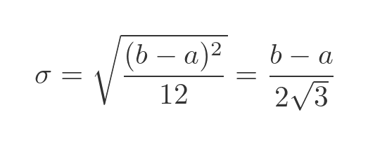
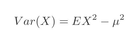
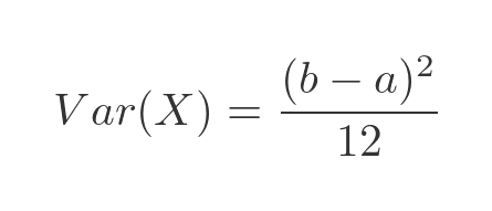
The variance of a distribution is the average of the squared difference of all the values from the mean. For the continuous uniform distribution, the variance is:

Again, we will prove this below. The standard deviation is a measure of how dispersed the values of the distribution are. It is defined as the square root of the variance:

Derivation of the mean

In general, the mean of any distribution E is given by:

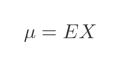
This expression is not quite as simple as it appears. E is a PDF, and X is a random variable, so how do we multiply them together?

Well, if we were dealing with a discrete distribution, for example, the mean score we would expect when throwing a dice many times, we would multiply each possible score (integers 1 to 6) by the probability of it occurring (1 in 6) to find the mean.

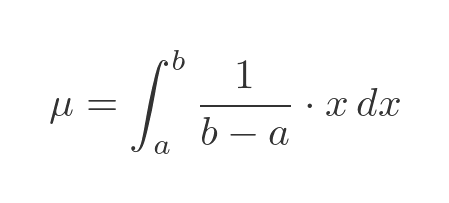
With a continuous distribution, we need to find the integral of the PDF function multiplied by x. The term EX is just shorthand for that integral. In our case the PDF is a constant value, 1/(b - a). But since the PDF is zero outside of the range a to b. we should only integrate EX over that range:

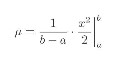
This is a simple integral, x times a constant, so the result is x squared over 2 times the constant:

Evaluating between a and b, and simplifying, gives:

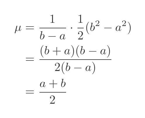
This, of course, is what we expected.

Derivation of the variance

In general, the variance of any distribution E is given by:

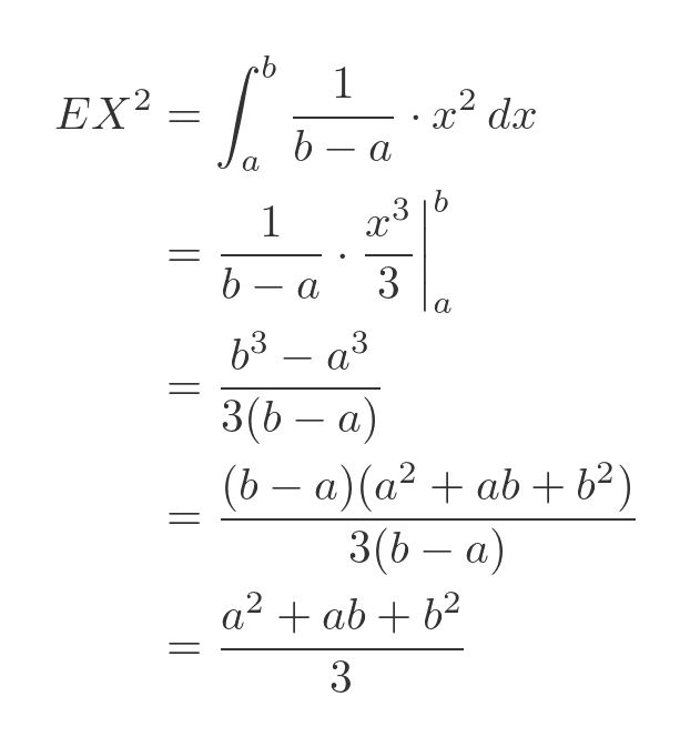
Again E times X squared is shorthand for the following integral:

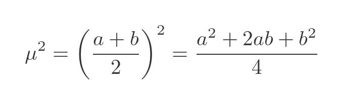
We know the mean, µ, from earlier so its square can be calculated:

Plugging both values into the expression for the variance gives:

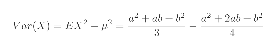
This can be simplified by multiplying out. It is straightforward but tedious so we will just give the final result here:

The standard deviation, by definition, is the square root of the variance, as we saw earlier.

The probability of a particular exact value is zero

We mentioned earlier that the probability of X taking any particular value in a continuous uniform distribution (or any continuous distribution) is zero. Why is that?

Taking the original wheel example, let's imagine we had a mathematically perfect wheel. When it stops, we can measure its exact position to as many decimal places as we like. So when we say it stops on exactly 0.4, we mean that it stops at 0.400000... to infinitely many decimal places.

We can represent every possible value by 0.xyz... where x is a digit from 0 to 9 representing the first digit in the wheel position, y is a digit from 0 to 9 representing the second digit in the wheel position, and so on.

If we consider all the possible outcomes, the first digit x can take any value from 0 to 9, with equal likelihood. So, in a particular spin of the wheel, the probability of x being zero is 1 in 10, or 0.1.

Similarly, the probability that y will be zero is 0.1. And the value of y is independent of the value of x. The same applies to z and every other digit.

Each digit is, in effect, an independent random variable. In order for the wheel to be exactly 0.4, we need every digit after the first to be zero. So we need infinitely many events to occur where each one has a probability of 0.1. This has zero chance of happening!

But of course, the wheel has to stop somewhere, and wherever it stops that exact combination of digits had zero chance of happening - and yet somehow it did! This is called the lottery paradox and will be a topic for another article.

In practical terms, no wheel is mathematically perfect, so we can only ever measure the position as being somewhere within a finite range.

See also

• Normal distribution
• Binomial distribution