Space-filling curves

In this article, we will look at space-filling curves. We will look at what a space-filling curve is, why they are so unusual, and the motivation for studying them. We will also look at some example space-filling curves and understand that they do indeed fill the whole space. Considering that a mathematical line has zero thickness, then using it to completely fill a two dimensional space is no mean feat!

We will take an intuitive approach, but will still attempt to address the mathematical problems that space-filling curves create.

Infinite sets

A lot of the motivation for studying space-filling curves comes from set theory, so we will quickly look at some relevant results here,

Georg Cantor was a mathematician who did a lot of work on set theory, including many important discoveries relating to infinite sets. He showed that infinite sets can be different sizes. For example, while there are infinitely many natural numbers, and there are infinitely many real numbers, there are actually far more real numbers than there are integers.

He also showed that some infinite sets are the same size, even when intuition suggests that they should not be. For example, the set of natural numbers and the set of even natural numbers are exactly the same size, even though intuitively you might expect the set of even numbers to be smaller. The size of a set is called its cardinality. For finite sets, the cardinality is a number (the number of elements in the set), but for infinite sets, the cardinality is represented by a symbol. The cardinality of the set of natural numbers is called aleph 0, written as ℵ₀.

But the discovery that we are interested in here is that the set of real numbers R is the same size as the set of all the pairs (x, y), where x and y are real numbers. This second set is called R². We can think of R as representing the real number line, and R² as representing the entire XY plane. Cantor tells us that the number of points on the real number line is the same as the number of points in the XY plane. The cardinality of each set is called aleph 1, written as ℵ₁.

What does this mean? It means that there is a one-to-one mapping between the points in R and R². Every point in R corresponds to exactly one point in R², and vice versa.

It can also be shown that the cardinality of the set of real numbers between 0.0 and 1.0 is aleph 1, so there are aleph 1 points on that line section. Also, the cardinality of the set of pairs of real numbers in a unit square is aleph 1, so there are aleph 1 points on that square:

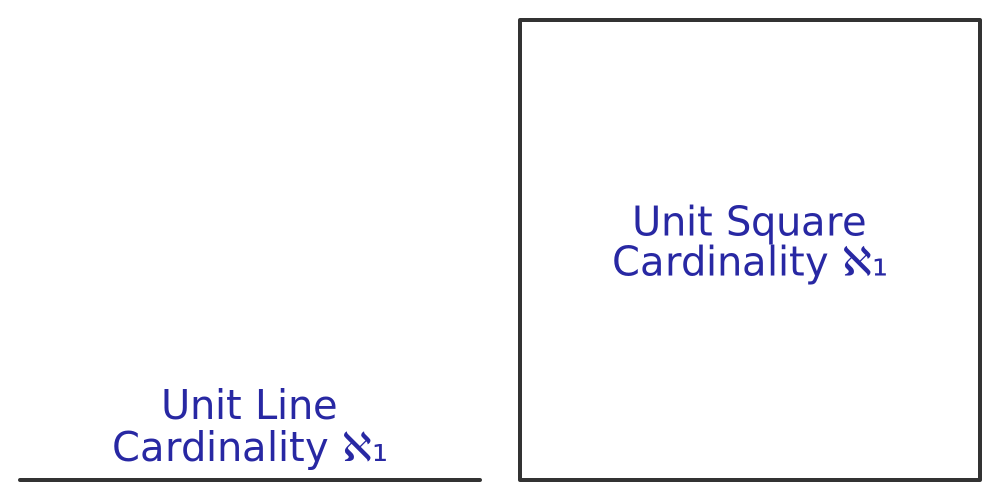
It is easier to visualise these finite regions, rather than infinite regions. And it is certainly easier to draw them, so we will use these regions in the rest of this article. But bear in mind that the results here can be extended to the infinite plane.

What is a space-filling curve?

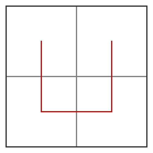
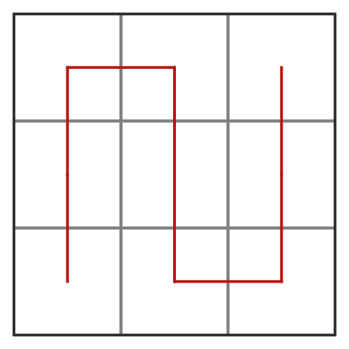
So this diagram shows two unit squares:

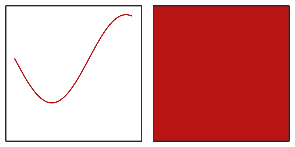
The square on the left shows an ordinary curve, that is, all the points that satisfy some simple relationship between x and y. We might say that this curve fills part of the space within the unit square. The one on the right shows what we might expect a space-filling curve to look like. It fills all of the space in the unit square.

But is that really true. It might look as if the curve on the left fills some of the area, but that is only because we have drawn it with a thick red line. The mathematical line corresponding the red line has zero thickness, therefore zero area, so it doesn't fill any of the square at all.

So the first curve fills none of the area. The space filling curve is longer, in fact much longer, but it still has zero thickness. So how could a sthat curve fill the whole area? How can we fill an area with a line that has zero width?

Alternative definition of a space-filling curve

If you think about it, we already know it is possible for something with no area to completely fill the unit square. The unit square is completely filled with (x, y) points. If you pick any position in the square, there will be a point there! But, of course, each point has zero area. When we talk about the points "filling" the area, perhaps what we really mean is that there is a point defined everywhere within the square.

We could define a space-filling curve in a similar way. If you pick any position in the square, the curve passes through that position. This removes any reference to the area filled by the curve.

Curves and functions

There is a third way to view this. The line on the left can be thought of as a mapping function:

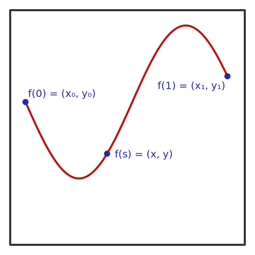
It maps a value s (between 0 and 1) onto a set of points (x, y). And since it is bijective, it also maps (x, y) values onto a value s, but only for those values that are on the curve.

The difference for a space-filling curve is that it works for every value point (x, y) in the unit square. In other words, it is a bijective mapping between the complete set of values on the real line [0, 1] and the complete set of points in the unit square. If you pick any point (x, y), it will map onto a position on the curve.

The Hilbert curve

There are numerous known space-filling curves. They are usually fractal in nature and can often be expressed as L systems. However, some of them were invented long before anyone started studying fractals.

One of the earliest attempts, and one that is still regarded as the most straightforward, is the Hilbert curve. The approach, taken by many space-filling curves, is to subdivide the unit square into smaller squares, defining a point at the centre of each smaller square. The curve is then formed by joining the centres of each square, according to some rule. We can then subdivide the squares further, usually applying the same rule recursively. The result is a curve that visits an ever larger set of points as the number of levels increases.

This is best seen by example. We first divide the main square into 4 smaller squares, and join the centres with a U-shaped red line, as shown:

For the next step, we divide the unit square into 16 smaller squares (in a 4 by 4 grid). Each quarter will be a 2 by 2 square, just like before. We can draw a red U-shape in each quarter, as shown below. Notice, however, that the top-left shape has been rotated 90 degrees counterclockwise, and the top-right shape has been similarly rotated clockwise (on the left):

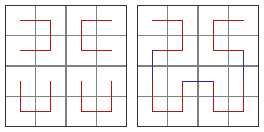
The RHS of the diagram above shows how the four separate curves can be joined, using the three lines indicated in blue. This creates a curve that visits every single square.

Notice that the number of vertices has increased by a factor of four (because we have created four copies of the original shape). The length of the red curve has doubled (there are four copies of the shape, but they are half the original size). The total length of the curve has also increased by the amount of the blue curve.

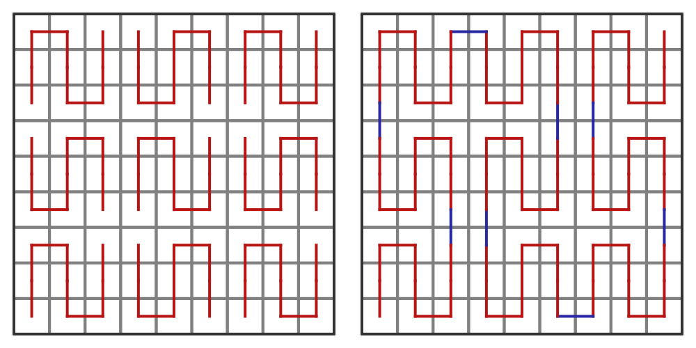
Below, we have divided the square into an 8 by 8 grid. We have duplicated the 4 by 4 pattern above into each quarter of the grid below, and again, we have rotated the top two quarters in the same way. These separate curves can be joined into one continuous curve by adding three lines shown in blue, shown on the right below:

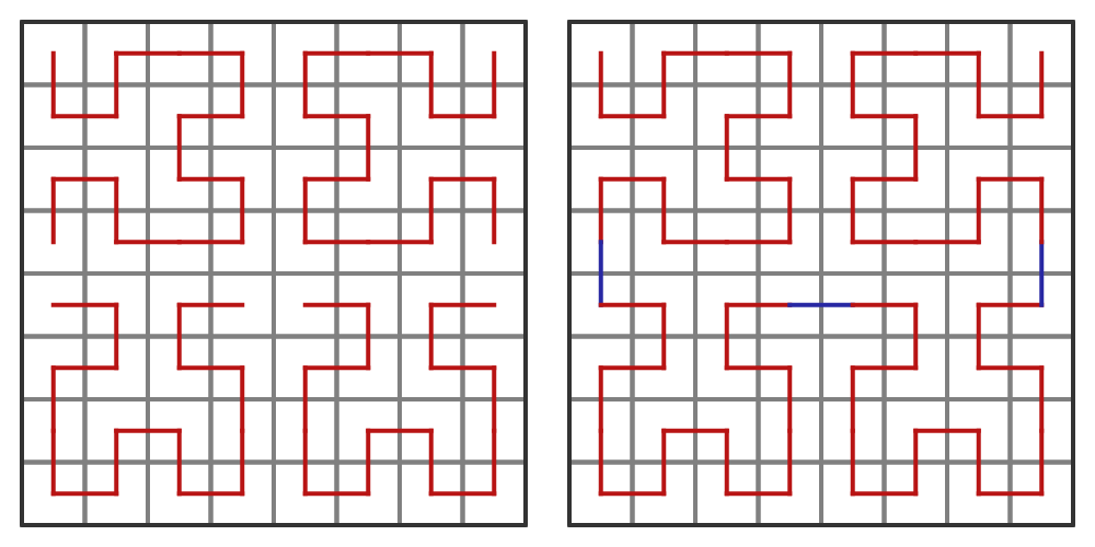
Once again, the number of vertices has increased by a factor of four and the length of the red curve has doubled. And again, we add the extra blue length, but the blue sections are smaller this time.

We can keep subdividing as many times as we like. Here we can see the 16 by 16 grid and the 32 by 32 grid:

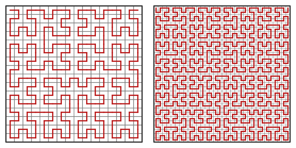
Each time we subdivide:

• the number of vertices in the curve increases by a factor of 4
• the length of the red part of the curve doubles (ignoring the blue part, which gets smaller and smaller on each iteration)

This means that as the number of iterations tends to infinity, the length of the curve and the number of vertices will both tend to infinity. That is what you would expect - a curve of finite length can't visit every point in the unit square.

Peano curve

There have been numerous other space-filling curves discovered over the years. We will look at another one here, the Peano curve, which was suggested before the Hilbert curve. It works in a similar way to the Hilbert curve, but with this initial shape:

Notice that this shape passes through the centres of nine sub-squares rather than four.

For the second iteration, we subdivide again, replicating the original shape nine times over a grid of 81 small squares:

This grid contains two orientations of the shape - the original shape and a mirrored shape. Since the basic shape has rotational symmetry of order two, it doesn't matter whether we mirror it vertically or horizontally (but not both!), it gives the same result. Alternate copies of the shape are either mirrored or not, in a checkerboard pattern.

The Peano curve was very clever in its own right and it inspired the Hilbert curve. But the Hilbert curve is preferred these days because it is simpler in several ways:

• The starting shape is simpler (three lines instead of five)
• It uses a subdivision of two rather than three
• It only requires three extra blue lines per iteration rather than eight

Mapping function

Part of the point of investigating space-filling curves is to demonstrate that it is possible to create a bijective function that maps a unit line onto a unit plane. We will see how this can be done using the Hilbert curve.

Here is the second iteration of the Hilbert curve. We have each point where the curve passes through the centre of one of the squares and numbered them 0 to 15:

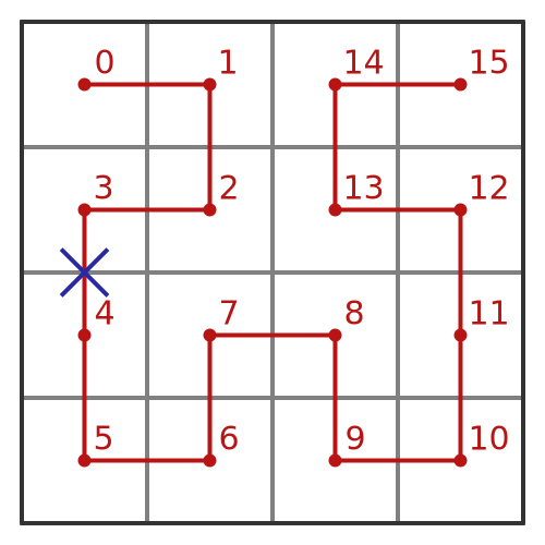
The blue cross represents a point in the curve. At any point on the curve, we can calculate:

• The position of the point on the curve. This is represented as a value between 0 and 1, where point 0 is position 0 and point 15 is position 1.
• The position of the point within the unit square, as (x, y) where x and y are between 0 and 1.

Let's do this for the blue cross. First, where is the cross on the line segment? We can see that it is halfway between points 3 and 4. This means that the curve length from point 0 to the cross is 3.5 segments. There are 15 segments, so each segment is 1/15 of the total length of the curve. This means that the cross is 7/30 of the way along the curve.

What about the position of the cross within the unit square? Each small square has a side of 1/4 (since the big square has a side of 1). So the x position of the cross is 1/8, and the y position is 1/2.

So our bijective function that maps the curve onto the unit square has the property that the position 7/30 maps onto the point (1/8, 1/2).

Now, with a lot more work, we could develop a formula that maps every point on the line onto a point in the unit square. It would be horrendous, but it could certainly be done.

We could do the same thing with the more detailed Hilbert curves we saw earlier, for example, the 32 by 32 version. That would be even more horrendous, but it is possible.

It is, in fact, possible to derive a general formula in terms of the number of iterations. This formula can be used to express the mapping function for the full Hilbert curve, with infinite iterations.

However, it takes the form of an infinite sum, so we can only approximate the actual values.

The important thing is that there is a bijective formula that maps the position along the Hilbert curve to the unit square.

Since the Hilbert curve is space-filling, this demonstrates that R and R² have the same cardinality.

A more direct mapping function

Finally, we will sketch out a simpler, more direct mapping function. Remember that all we really need to show is that every real number in the range 0 to 1 maps onto a unique point in the unit square, and vice versa.

As an illustration, we can take any point in the unit square. It is easier to illustrate the point when the coordinates are irrational numbers, so we will choose this point:

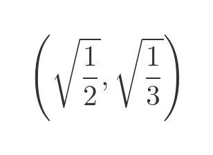
The values of these two roots are:

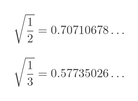
We convert these two numbers into a single number by interleaving the digits of the two numbers above. We take the first digit from the first number, then the first digit from the second number, then he second digit from the first number, then the second digit from the second number, and so on. Like this:

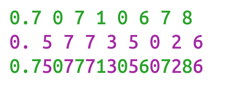
This gives a final number of:

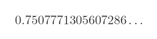
This number contains all the digits of both numbers. That means that if either input number was different in any digit, then the resulting number would be different.

Also, of course, if we are given the final number, we can find the two input numbers by separating out the digits. So the function is bijective.

There are a couple of problems with this approach, which we won't go into any further here. The main problem relates to numbers of this form:

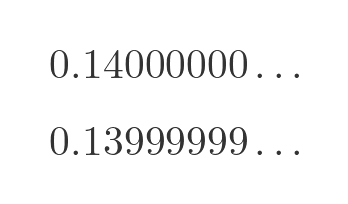
These two numbers are equal, because 0.00999999... is equivalent to 0.01. But the two forms of the number give completely different results when interleaved with a second number. There are ways to get around this and other small problems, but we won't cover them here.